Sizing assumptions for solutions with Erasure Coding (EC-X)

A common question recently has been how should I size a solution with Erasure Coding (EC-X) from a capacity perspective.

As a general rule, any-time I size a solution using data reduction technology including Compression, De-duplication and Erasure Coding, I always size on the conservative side as the capacity savings these technologies provide can vary greatly from workload to workload and customer to customer.

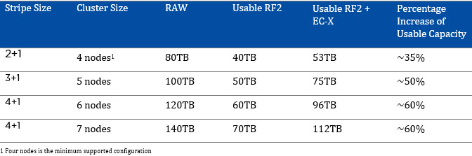
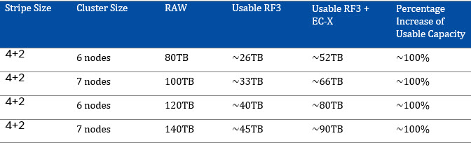
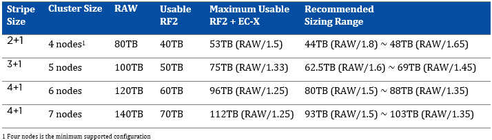
To assist with sizing, I have created the below tables showing the RAW capacity, usable capacity based on RF, Maximum usable with EC-X and my recommended sizing range.

You will note the recommended sizing is a range between roughly 50-80% of the theoretical maximum capacity EC-X can provide.

This is because EC-X is a post process and is only applied to Write Cold data as per my earlier post: What I/O will Nutanix Erasure coding (EC-X) take effect on?

This means it is unlikely all data will have EC-X applied and as a result, the usable capacity will generally be less than the maximum.

The following are general recommendations, which may not be applicable to every environment. For example, if your workload is heavy on “overwrites”, your EC-X capacity savings will likely be minimal, but for general server workloads, the below can be used as a rule of thumb:

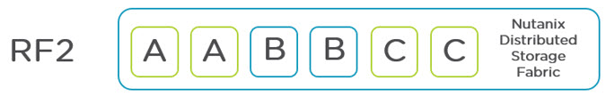
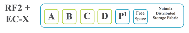
RF2 + EC-X Recommended Sizing Range

RF2ECXsizingassumptionsrange


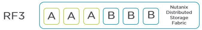
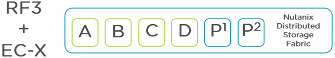
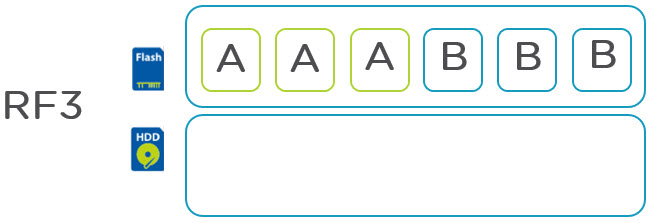
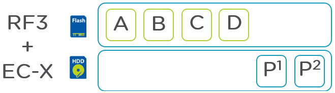
RF3 + EC-X Recommended Sizing RangeRF3ECXsizingassumptionsrange

If you want to be conservative with sizing, I recommend choosing the lower value in the sizing range. If you are happy to be less conservative then the higher number in the range can be used.

If you decide to size based on a number outside the recommended range, please document the assumed EC-X data reduction ratio and a risk that states in the event EC-X savings are less than “insert your value here” additional nodes will need to be purchased.

Tip: Always size for at least N+1 at the capacity layer, meaning if your largest node is 10TB RAW and with EC-X and RF2 you expect to have for example 7.5TB usable, that your container is configured with an “Advertised Capacity” at least N-1 capacity of the storage pool. (Or N-2 for clusters using RF3)

I hope you find this helpful when sizing your Nutanix environments.

RF2 & RF3 Usable Capacity with Erasure Coding (EC-X)

Over the past few weeks with the release of Acropolis base version 4.5 (formally known as NOS) on the horizon there has been a lot of interest in Erasure Coding (EC-X) which was announced at Nutanix .NEXT conference in June this year.

The most common questions are how does EC-X increase the effective SSD tier capacity and the overall cluster usable capacity. This post aims to cover these questions.

Resiliency Factor 2 (RF2) & Erasure Coding

Resiliency Factor 2 ensures that two copies of all data are written to persistent media prior to being acknowledged to the guest operating system. This ensures at N+1 level of redundancy which translates to being able to tolerate a single failure.

RF2 provides a usable capacity of ~50% of RAW.

The below figure shows an example of RF2 where six blocks store three pieces of data in a redundant fashion. In this configuration a single SSD/HDD or node can be lost without impacting data availability.

RF2normal

Now let’s take a look at how the same 6 blocks will be utilized with Erasure Coding enabled:

RF2plusECX

As we can see, we are now able to store four pieces of data (A,B,C,D) with single parity to ensure data can be rebuilt in the event of a drive or node failure. As with standard RF2, an RF2 + EC-X configuration can also tolerate a single SSD/HDD or node can be lost without impacting data availability. We also free up space to be used for another EC-X stripe.

As a result, the usable capacity increases from approx. 50% usable up to 80% usable for clusters of six (6) or larger.

The following table shows the maximum usable capacity for RF2 + EC-X based on cluster size:

Note: Assumes 20TB RAW per node

RF2table

Resiliency Factor 3 (RF3) & Erasure Coding

Resiliency Factor 3 ensures that three copies of all data are written to persistent media prior to being acknowledged to the guest operating system. This ensures at N+2 level of redundancy which translates to being able to tolerate two concurrent SSD/HDD or node failures.

RF3 provides a usable capacity of ~33% of RAW.

The below figure shows an example of RF3 where six blocks store two pieces of data in a redundant fashion. In this configuration the environment can tolerate two concurrent SSD/HDD or node failures without impacting data availability.

RF3normal

Now let’s take a look at how the same 6 blocks will be utilized with Erasure Coding enabled:

RF3ECX

Similar to the RF2 example, we can see we are now able to store more data with the same level of redundancy. In this case, five pieces of data (A,B,C, D) with dual parity to ensure data can be rebuilt in the event of dual concurrent drive or node failures. As with standard RF3, an RF3 + EC-X provides an N+2 level of availability while providing higher usable capacity.

The following table shows the usable capacity for RF3 + EC-X based on cluster size:

Note: Assumes 20TB RAW per node

RF3ECXtable

EC-X Parity Placement

To further increase the effective capacity of the SSD tier and there for supporting larger working set sizes with all flash performance, the Parity for containers with EC-X enabled is stored on the SATA tier.

The following figure shows a standard RF3 deployment:

RF3parityNormal

As we can see, 6 blocks of storage contain just 2 actual pieces of user data all of which reside in the SSD tier.

With RF3 + EC-X the same 6 blocks of storage contain 4 pieces of user data thus increasing the effective capacity of the SSD tier by 100% due to being able to store 4 piece of data compare to two with RF3. In addition the effective SSD capacity is further increased by moving the 2 parity blocks to SATA freeing up a further 33% SSD tier capacity.

RF3ECXparity

I hope that explains how EC-X works and why its such an advantage for Nutanix current and futures customers.

Related Articles:

  1. Nutanix Erasure Coding Deep Dive
  2. Increasing resiliency of large clusters with Erasure Coding
  3. What I/O will EC-X take effect on?
  4. Sizing assumptions for solutions with Erasure Coding (EC-X)


Uploading ISOs & VM Images to Acropolis Hypervisor (AHV)

A common question is how do I upload an ISO or Virtual machine image to the Acropolis Hypervisor, well in NOS 4.5 this task just got radically simpler.

The below shows the “Home” screen in PRISM UI. As we can see in the top left we are running the Acropolis Hypervisor (AHV) version 20150616.

By clicking the gear wheel at the top right, we can then access the “Image Configuration” menu.PRISMHomeImageService

The “Image configuration” menu is a quick and easy way to upload ISOs and Virtual Machine images to Acropolis.

Below we can see its a very simple process, simply give the Image a name along with annotation, select from a drop-down list the Image type, being ISO or Disk (RAW format, .img) and then select the image source, either from a URL or by uploading a file from your machine.

CreateImage

Once you have selected your ISO or Disk, hit save and the image will be uploaded and the status of the upload will be shown as per the below:

CreateImageUploading

Once its completed, PRISM shows the following Summary:

ImageConfigurationSuccess

Now when you create a new VM, you will be able to select “Clone from Image Service” and select the ISO Image from a drop-down list. How simple is that!

CDROMimageservice

Simple as that! Now you can boot your VM and start using the ISO. The same process can also be used to upload VM disk images.