How to successfully Virtualize MS Exchange – Part 17 – Virtual Machine Storage Configuration

In addition to Part 16 where we discussed Virtual Disk Provisioning options and recommendations, In this part we will cover how to optimally configure a Virtual Machine for an Exchange MBX/MSR workload from a virtual storage controller perspective.

Once you have made the decision on storage platform, and assuming you have chosen to use VMFS or NFS datastores (and not iSCSI in-Guest or RDMs), then this article is for you.

Virtual Machines just like physical servers, have SCSI controllers (albeit virtual) and ESXi has a number of options to choose from which include:

1. BusLogic Parallel
2. LSI Logic Parallel
3. LSI Logic SAS
4. Paravirtual SCSI (PVSCSI)
5. AHCI SATA Controller

By default when creating a new virtual machine the default adapter for Windows 2008 and 2012 is “LSI Logic SAS” because Windows does not have the PVSCSI driver by default.

BusLogic ParallelLSI Logic Parallel adapters are not recommended for Windows 2008/2012 as they are legacy controllers with lower performance, as such I will not cover these in any more detail as they are irrelevant to Exchange deployments.

Instead I will cover the LSI Logic SASAHCI SATA Controller and Paravirtual SCSI (PVSCSI) adapters.

Starting with LSI Logic SAS,

This is the default controller for Windows 2008/2012 VMs, as a result, it is very common to see Exchange deployments using this controller. It has good performance and works out of the box with a Windows install without requiring drivers.

Advantages:

1. The default Controller for Windows 2008/2012
2. No need for manually inserting drivers to install Windows
3. Higher performance than AHCI SATA controller

Disadvantages:

1. Lower performance than PVSCSI
2. Higher CPU overheads in Guest compared to PVSCSI
3. Higher latency than PVSCSI
4. Lower maximum number of VMDKs supported per controller (15) compared to AHCI SATA (30)

Next let’s discuss the AHCI SATA Controller.

The AHCI SATA controller is new in vSphere 5.5 and is only supported in Virtual Machines with Hardware version 10. The SATA controller can be used on its own or in addition to LSI or PVSCSI controllers to provide additional VMDKs / Capacity which increases a single VMs maximum capacity from ~3.7PB to over 11PB.

Advantages:

1. Can support 30 VMDKs per Controller (120 total) compared to 15 for LSI / PVSCSI
2. Can be used in addition to PVSCSI controllers to provide more storage performance and capacity per Exchange VM (if required)
3. High capacity supported per controller than LSI Logic / PVSCSI

Disadvantages:

1. Higher CPU utilization per IO compared to LSI / PVSCSI options
2. Lower overall performance compared to LSI and PVSCSI
3. Higher latency compared to LSI and PVSCS

And Finally the Paravirtual SCSI Controller.

The PVSCSI controller is the highest performing controller and has been supported since ESXi 4.0 and are design for high performance storage environments and are available for virtual machines running hardware version 7 and later.

Advantages:

1. Performance , Performance , Performance. Oh yeah and did I mention performance?
2. Lower Latency and Higher IOPS compared to other controllers
3. Lower CPU overhead on the Guest OS (and therefore ESXi)
4. More CPU is available for Exchange due to lower CPU overheads

Disadvantages:

1. Windows Failover Clustering is not supported, but this has no impact on MS Exchange including DAG deployments.
2. PVSCSI is not the default and requires inserting drivers into the Windows installation OR the VM to be built on LSI Logic SAS and once VMware Tools is installed, swapping to PVSCSI.
3. Lower maximum VMDKs supported per controller (15) compared to AHCI SATA (30)

Performance Comparison

From a performance perspective, Michael Webster (VCDX#66) wrote this great post “VMware vSphere 5.5 Virtual Storage Adapter Performance” and produced the following graph showing a comparison between SATA, LSI Logic SAS and PVSCSI controllers from an IOPS, Latency perspective.

VMware-vSphere-5.5-Virtual-Storage-Adapter-Performance

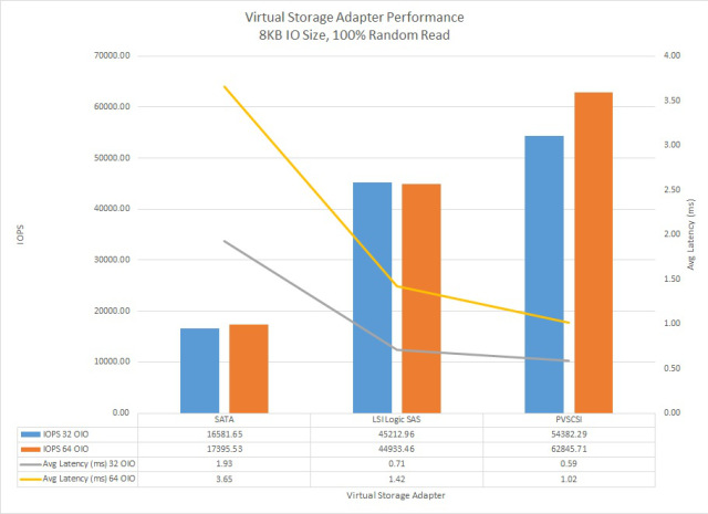
As we can see, the PVSCSI adapter has significantly lower latency and higher IOPS than the SATA and LSILogic SAS controllers even when running on the same underlying storage.

While the Microsoft Exchange team have managed to successfully reduce I/O throughout the versions (2007-2013) the performance advantages also have a positive benefit on vCPU utilization.

Michael’s post states:

It (PVSCSI Controller) also had the lowest CPU usage. During the 32 OIO test SATA showed 52% CPU utilization vs 45% for LSI Logic SAS and 33% for PVSCSI.

What this means is less CPU utilization is used for I/O and lower average latency means more CPU is available for MS Exchange along with less CPU WAIT time (where the CPU is waiting for IO to complete before continuing). This means your onto a winner especially considering Exchange 2013 is very CPU intensive.

Which Controller should be used for Exchange VMs?

VMware have published the KB article “Do I choose the PVSCSI or LSI Logic virtual adapter on ESX\ESXi 4.0 for non-IO intensive workloads? (1017652)” which in summary explains:

The test results show that PVSCSI is better than LSI Logic, except under one condition–the virtual machine is performing less than 2,000 IOPS and issuing greater than 4 outstanding I/Os. This issue is fixed in vSphere 4.1 and later version, so that the PVSCSI virtual adapter can be used with good performance, even under this condition.


As the one caveat prior to vSphere 4.1 where LSI Logic can outperform PVSCSI, there are no significant downsides to using the PVSCSI compared to LSI as such, I recommend always using (multiple) PVSCSI adapters.

Now that we have decided on the PVSCSI adapter, what’s next?

As with physical servers, Virtual SCSI controllers including PVSCSI have their limits in terms of performance and scalability. To ensure maximum scalability, performance and low latency, multiple PVSCSI adapters should be used with all VMDKs evenly spread over the PVSCSI adapters as recommended in Part 11.

To do this, when adding a VMDK to the Exchange VM, ensure you select a different SCSI controller (which are created automatically on demand) by using the drop down box “Virtual Device Node” and selecting for example SCSI (1:0) as shown below.

MSRVMPVSCSI10

For subsequent VMDKs you must then select SCSI (2:0) as shown below.

MSRVMPVSCSI20

And then SCSI (3:0)

MSRVMPVSCSI30

For the forth VMDK, you then select SCSI (0:1) because SCSI (0:0) is taken by the VMDK used for the guest OS.

MSRVMPVSCSI01

Repeat the above process until you have sufficient VMDKs for your Exchange server VM.

The following illustrates my recommended configuration showing how to configure a VM supporting 8 database drives and 8 log drives.PVSCSIVMDKs

The above configuration will ensure maximum storage performance and can be expanded in the same configuration to support more than 3 times the number of databases + logs shown above and as such it is suitable for even very large (scale-up) Exchange MBX/MSR VMs.

For example, if each VMDK in the above configuration was just 4TB in size it would give you 64TB usable capacity and the VM can be scaled more than 3x the number of VMDKs.

Note: VMDKs can scale to 62TB (from vSphere 5.5) each although this may result in reduced performance.

TIP: Don’t forget to spread VMDKs evenly across datastores as per the recommendation in Part 11.

Recommendations for Exchange VM Storage Configuration:

1. Use multiple Paravirtual SCSI (PVSCSI) Adapters.
2. Use one VMDK per Database or Logs
3. Spread VMDKs evenly across multiple PVSCSI adapters
4. Spread VMDKs evenly across multiple datastores when using VMFS datastores
5. Spread VMDKs evenly across multiple datastores when using NFS datastores ensuring NFS datastores are served via multiple NAS controllers
6. Use more VMDKs as opposed to fewer larger VMDKs
7. Format NTFS volumes with an Allocation Unit Size of 64k
8. Keep it simple, do not mix virtual SCSI controller types.

Back to the Index of How to successfully Virtualize MS Exchange.

Scaling problems with traditional shared storage

At VMware vForum Sydney this week I presented “Taking vSphere to the next level with converged infrastructure”.

Firstly, I wanted to thank everyone who attended the session, it was a great turnout and during the Q&A there were a ton of great questions.

One part of the presentation I got a lot of feedback on was when I spoke about Performance and Scaling and how this is a major issue with traditional shared storage.

So for those who couldn’t attend the session, I decided to create this post.

So lets start with a traditional environment with two VMware ESXi hosts, connected via FC or IP to a Storage array. In this example the storage controllers have a combined capability of 100K IOPS.

50kIOPS

As we have two (2) ESXi hosts, if we divide the performance capabilities of the storage controllers between the two hosts we get 50K IOPS per node.

This is an example of what I have typically seen in customer sites, and day 1, and performance normally meets the customers requirements.

As environments tend to grow over time, the most common thing to expand is the compute layer, so the below shows what happens when a third ESXi host is added to the cluster, and connected to the SAN.

33KIOPS

The 100K IOPS is now divided by 3, and each ESXi host now has 33K IOPS.

This isn’t really what customers expect when they add additional servers to an environment, but in reality, the storage performance is further divided between ESXi hosts and results in less IOPS per host in the best case scenario. Worst case scenario is the additional workloads on the third host create contention, and each host may have even less IOPS available to it.

But wait, there’s more!

What happens when we add a forth host? We further reduce the storage performance per ESXi host to 25K IOPS as shown below, which is HALF the original performance.

25KIOPS

At this stage, the customers performance is generally significantly impacted, and there is no easy or cost effective resolution to the problem.

….. and when we add a fifth host? We continue to reduce the storage performance per ESXi host to 20K IOPS which is less than half its original performance.

20KIOPS

So at this stage, some of you may be thinking, “yeah yeah, but I would also scale my storage by adding disk shelves.”

So lets add a disk shelf and see what happens.

20KIOPSAddDiskShelf

We still only have 100K IOPS capable storage controllers, so we don’t get any additional IOPS to our ESXi hosts, the result of adding the additional disk shelf is REDUCED performance per GB!

Make sure when your looking at implementing, upgrading or replacing your storage solution that it can actually scale both performance (IOPS/throughput) AND capacity in a linear fashion,otherwise your environment will to some extent be impacted by what I have explained above. The only ways to avoid the above is to oversize your storage day 1, but even if you do this, over time your environment will appear to become slower (and your CAPEX will be very high).

Also, consider the scaling increments, as a solutions ability to scale should not require you to replace controllers or disks, or have a maximum number of controllers in the cluster. it also should scale in both small, medium and large increments depending on the requirements of the customer.

This is why I believe scale out shared nothing architecture will be the architecture of the future and it has already been proven by the likes of Google, Facebook and Twitter, and now brought to market by Nutanix.

Traditional storage, no matter how intelligent does not scale linearly or granularly enough. This results in complexity in architecture of storage solutions for environments which grow over time and lead to customers spending more money up front when the investment may not be realised for 2-5 years.

I’d prefer to be able to Start small with as little as 3 nodes, and scale one node at a time (regardless of node model ie: NX1000 , NX3000 , NX6000) to meet my customers requirements and never have to replace hardware just to get more performance or capacity.

Here is a summary of the Nutanix scaling capabilities, where you can scale Compute heavy, storage heavy or a mix of both as required.

ScaingSolution

Data Locality & Why is important for vSphere DRS clusters

I have had a lot of people reach out to me since VMworld SFO, where I was interviewed by Eric Sloof (@esloof) on VMworldTV (interview can be seen here) about Nutanix.

So I thought I would expand on the topic of Data Locality and why it is so important for vSphere DRS clusters to maintain consistent high performance and low latency.

So first, the below diagram shows three (3) Nutanix nodes, and one (1) Guest VM.

NutanixLocalRead

The guest VM is reading data from the local storage in the Nutanix node and as a result this read access is very fast. The read I/O will be served from one of 4 places.

1. Extent Cache (DRAM – For “Active Working Set”)
2. Local SSD (For “Active Working Set”)
3. Local SATA (Only for “Cold” data)

and the forth we will discuss is a moment.

So as a result for Read I/O

1. There is no dependency on a Storage Area Network (FCoE, IP, FC etc)
2. Read I/O from one node does not contend with another node
3. Read I/O is very low latency as it does not leave the ESXi host
4. More Network bandwidth is available for Virtual Machine traffic, ESXi Mgmt, vMotion , FT etc

But wait, the what happens if DRS (or a vSphere admin) vMotion’s a VM to another node? – I’m glad you asked!

The below shows what happens immediately after a vMotion

NutanixAftervmotion

As you can see, only the Purple data is local to the new node, so transparently to the virtual machine, if/when remote data is required by the VM (ie: The VMs “Active Working Set”) the Nutanix controller VM (CVM) will get the requested data over the 10GB Network in 1MB extents. (It does not do a bulk movement or “Storage vMotion” type movement of all the VMs data EVER!)

And, all future Write I/O will be written local, so future Read I/O will all be local by default.

So, the worst case scenario for a read I/O in a Nutanix environment, is that the required data is not available locally and the CVM will access the data over a 10GB network.

This scenario will only occur in situations where

1. Maintenance is occurring and hosts are rebooted
2. A Host Failure (HA restarts VM on another node)
3. Following a vMotion

Generally in BAU (Business as Usual) operation Read I/O should be local in the high 90% range.

So the worst case scenario for Read I/O on a vSphere Cluster running on Nutanix, is actually the Best case scenario for a traditional storage array, because in a traditional array all data is accessed over some form of storage network and generally via a small number of controllers.

It is important to note, the Nutanix DFS (Distributed File System) only accesses data over the network when its required by the VM at a granular (1MB extent) level. So only the “Active Working Set” will be accessed over the 10Gb network, before being copied locally, again in 1MB extents. So if the data is not “Active” having it remotely does not impact performance at all so moving the data would create an overhead on the environment for no benefit.

In the event 90% of a VMs data is on a remote node, but the “Active Working Set” is local, read performance will all be at local speeds, again from Extent Cache (DRAM), Local SSD or Local SATA (for “cold” data).

Now some vendors are working on or have some local caching capabilities which in my experience are not widely deployed and have various caveats such as Operating System version, and in guest drivers, but for the vast majority of environments today, these technologies are not deployed.

The Nutanix DFS has data locality built in, it works with any hypervisor , Guest OS and does not require any configuration.

So now you know why ensuring the Active Working Set (data) is as close to the VM is essential for consistent high performance and low latency.

Related Articles

1. Write I/O Performance & High Availability in a scale-out Distributed File System