
I’ve been doing some testing recently with Nutanix latest GA code (AOS 5.8) and I decided to do some quick MS Exchange Jetstress performance tests as part of a larger piece of work.
In short I wanted to check how well Exchange storage performance scaled so I performed three tests. I started with 4 threads, then increased to 8 and finally to 12 threads using Jetress with Exchange 2016 ESE database modules.
For this testing I disabled the Nutanix in memory read cache to ensure all read IO is serviced by the physical SSDs so the result is not artificially improved from cache.
I also disabled Compression, Erasure Coding and Deduplication as these also artificially improve performance due to Jetstress data being highly compressible & dedupable.
The hardware used was a NX-8150 with 6 x SSDs and Intel Broadwell processors. This is why the database size was only 1.7TB as that’s just below the total usable capacity of the node. The performance over larger database sizes remains the same when the metadata cache (in the Nutanix Controller VM) is sized for the desired working set size as shown by our ESRP certification.
The hypervisor is Acropolis Hypervisor (AHV) which is fully certified for Microsoft Windows under the MS SVVP programme as well as MS ESRP certified for MS Exchange.
So here is the result for 4 threads.
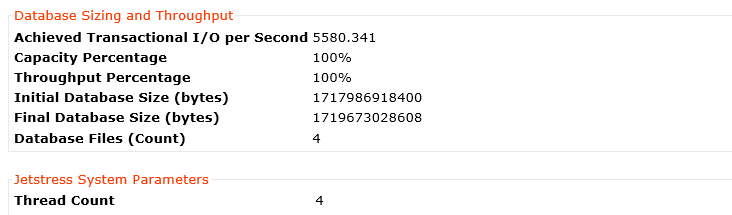
5580 IOPS with just 4 threads is very good performance and is sufficient for at least five thousand mailboxes with hundreds of messages per day which is maximum recommended active users per Exchange MSR server.
The next question is: What’s the latency for the database reads and log writes? (These are two of the critical performance metrics for Jetstress Pass/Fail results)
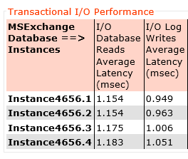
Here we can see log write latency average across all four log drives is below 1ms (0.99ms) and database read latency at 1.16ms.
Next up, here is the result for 8 threads.
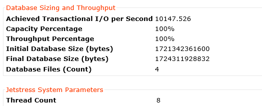
10147 IOPS with 8 threads is excellent performance and shows Nutanix easily has headroom for more than ten-thousand mailboxes with hundreds of messages per day which easily exceeds the requirements for the maximum recommended active users per Exchange MSR server.
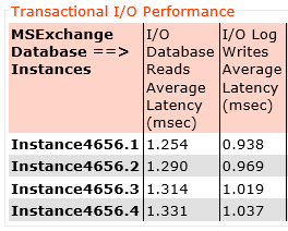
Again let’s check out the latency, Here we can see log write latency average across all four log drives is still below 1ms (0.99ms) and database read latency at 1.29ms. That’s just 0.13ms higher latency for reads and exactly the same write latency while achieving almost DOUBLE the IOPS.
Lastly here is the result for 12 threads.
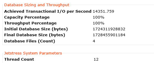
14351 IOPS with 12 threads proves how scalable the Nutanix platform is as this is almost a linear increase in IOPS.
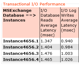
Again let’s check out the latency, Here we can see log write latency average across all four log drives is still below 1ms (0.98ms) and database read latency at 1.42ms. That’s just 0.14ms higher latency for reads and slightly lower write latency while achieving almost linear improvement in IOPS.
Summary:
Nutanix provides extremely high, predictable performance for even the most demanding MS Exchange environments.