Splitting SQL datafiles across multiple VMDKs for optimal VM performance

After recently helping multiple customers resolve performance issues with vBCA workloads by configuring multiple PVSCSI adapters and spreading workloads across multiple VMDKs, I wrote: SQL and Exchange performance in a virtual machine.

The post talked about how you should use multiple PVSCSI adapters with multiple VMDKs spread evenly across the adapters to achieve optimal performance and reduce overheads.

But what about if you only have a single SQL database. Can we split it across multiple VMDKs and importantly, can we do this without downtime?

The answer to both, thankfully is Yes!

The below is an example of a worst case scenario for a SQL server database. A single VMDK (using a single SCSI controller) hosting the Operating System, Database and Logs, especially when it’s a business critical application.

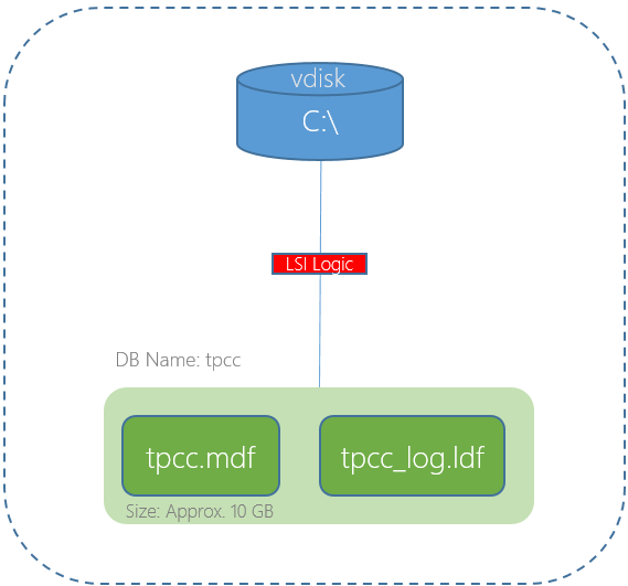
In the above scenario the single virtual SCSI controller and/or the single VMDK could both result in lower than expected performance.

We have learned earlier that using multiple PVSCSI adapters and VMDKs is the best way to deploy a high performance solution. The below is an example deployment where the OS , Pagefile and SQL binaries are using one virtual controller and VMDK, then four VMDKs for database files are hosted by a further two PVSCSI controllers and the logs are hosted by a fourth PVSCSI controller and VMDK.

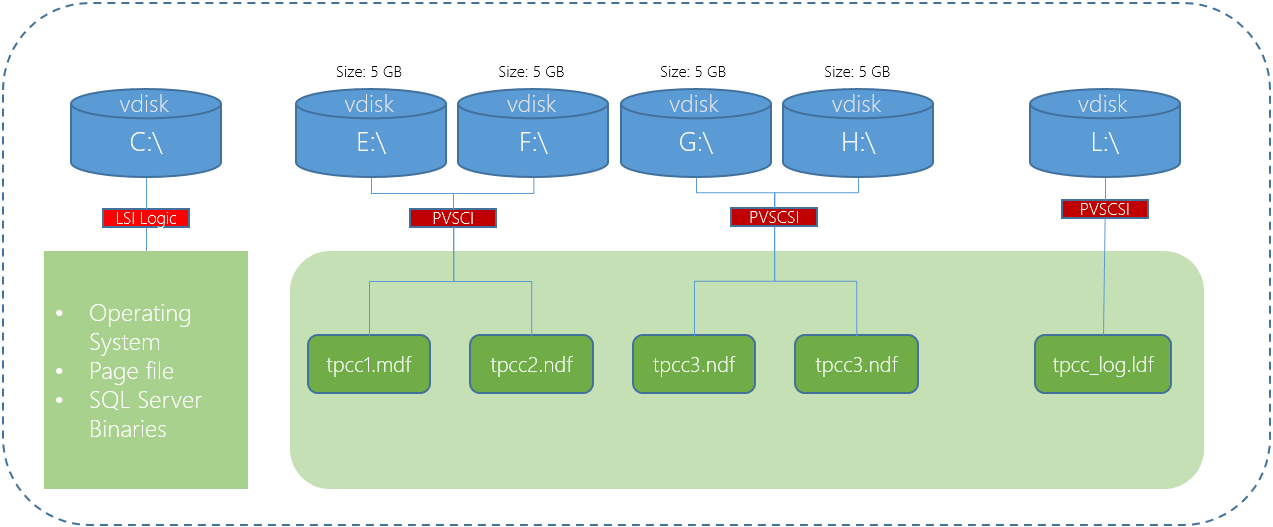
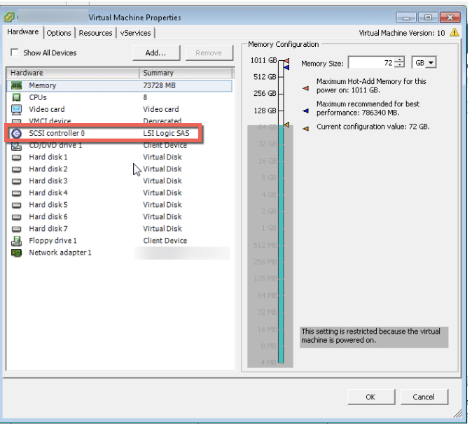
In the above diagram the C:\ is using a LSI Logic controller which in most cases does not constraint performance, however since it’s very easy to change to a PVSCSI controller and there are no significant downsides, I recommend standardizing on PVSCSI.

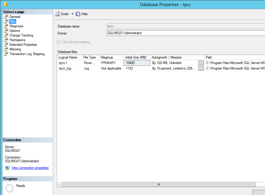
Now if we look at our current database, we can see it has one database file and one log file as shown below.

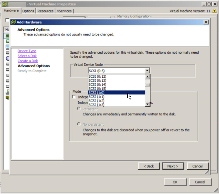
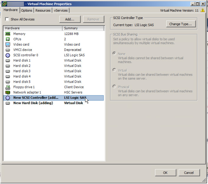
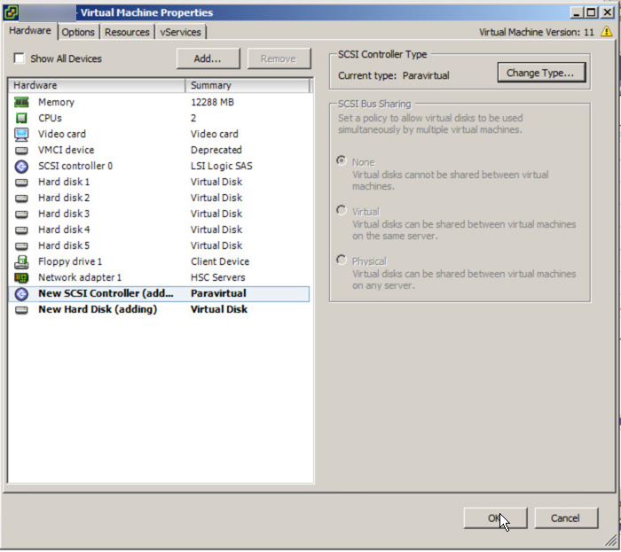
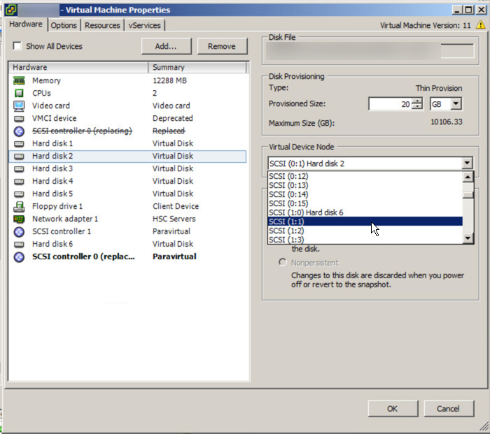
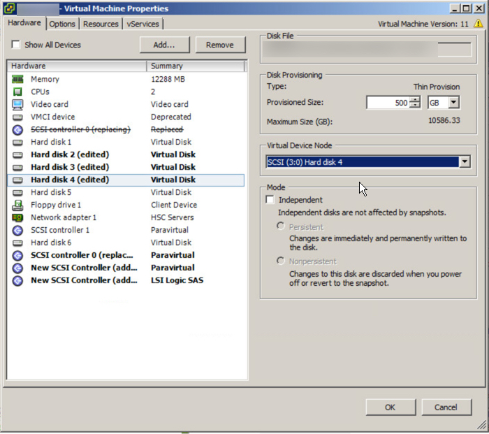
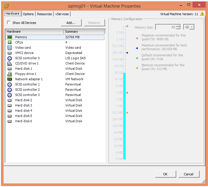
The first step is the update the Virtual machines disk layout as describe in the aforementioned article which should end up looking like the below:

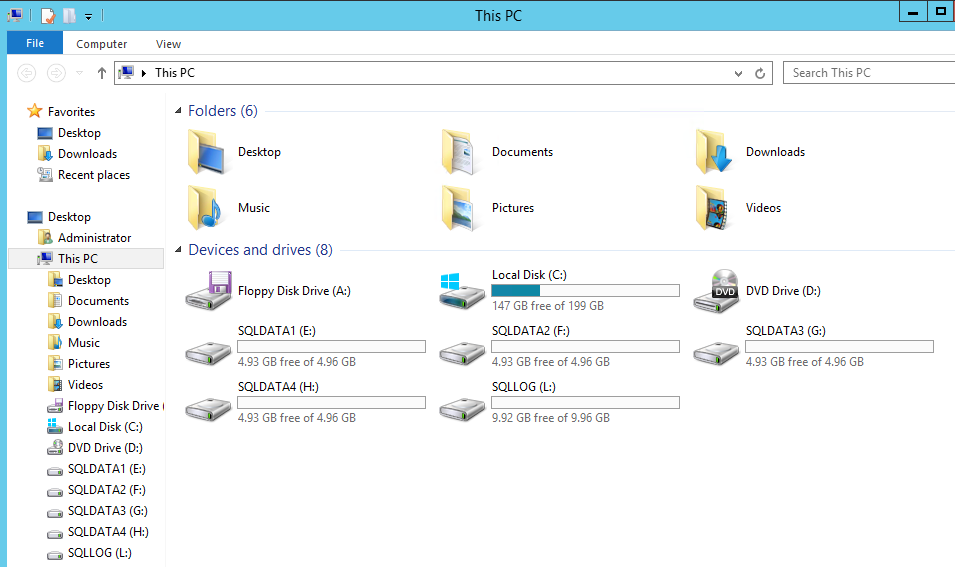
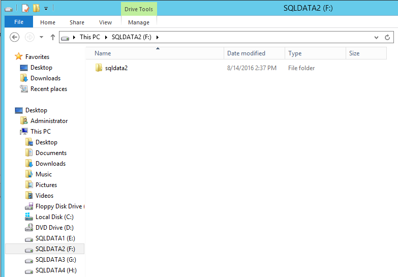
Next we go into Disk manager to rescan for the new storage devices, mark the drives are online, then format them with a 64k Allocation size which is optimal for databases. Once this is done you should check My Computer and see something similar to the below:

Next I recommend creating a directory for the database and log files rather than using the root directory so each drive should have a new folder as per the example below.

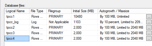
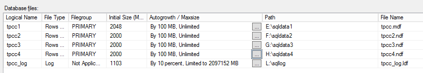
Next step is to create the new database files on each of new drives as shown below.

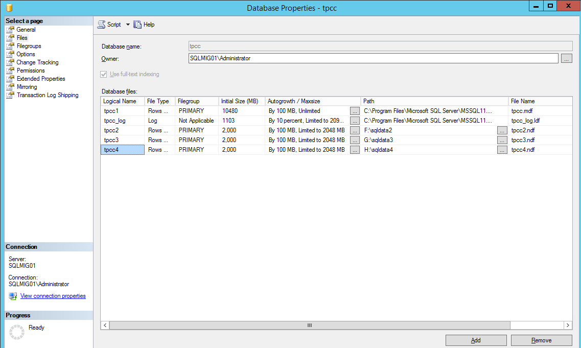
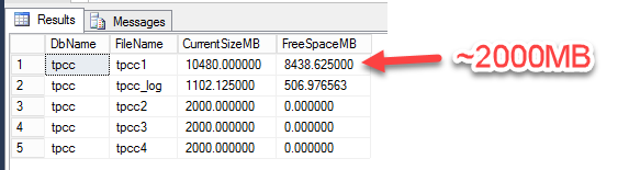
If the size of the original database is for example 10GB with say 2GB free space and you plan to split the database across 4 drives, then each of the new databases should be sized at no more than 2GB each to begin with. This prepares us to shrink the original DB and helps ensure the data is evenly spread across the new database files.

In the above screenshot, we can see the databases are limited to 2000MB, this is on purpose as we don’t want the database files expanding which can result in an uneven spread of data during the redistribution process I will cover later.

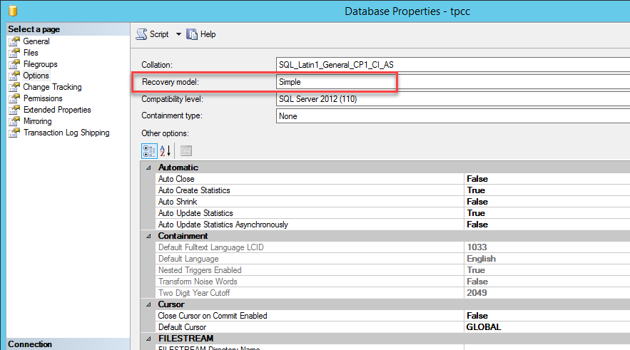
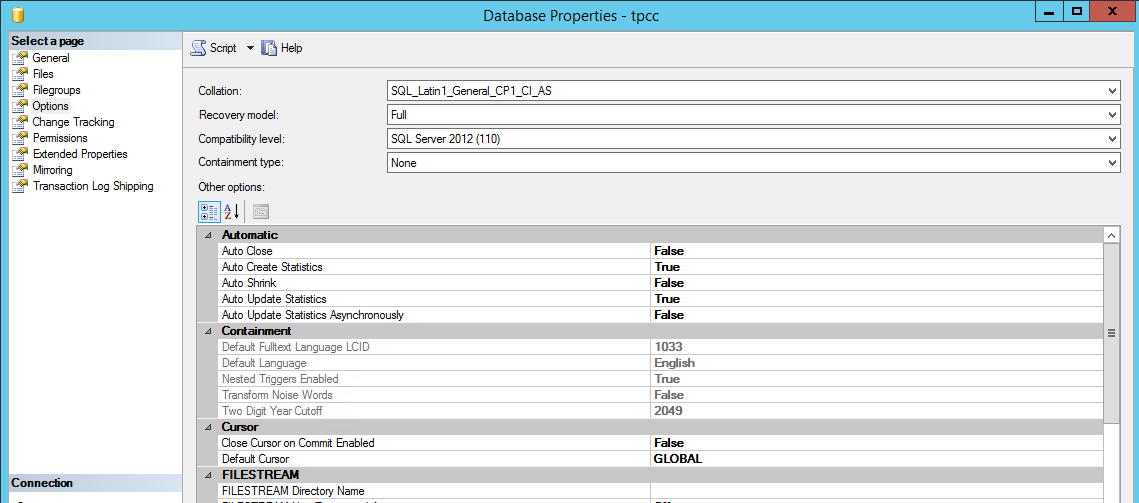
Switch the Recovery mode of Database to SIMPLE

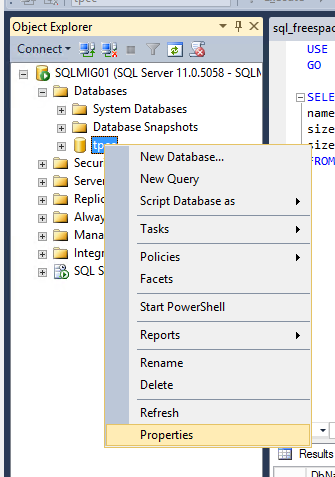
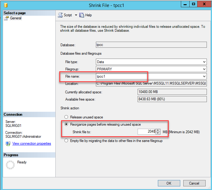
Now go to the database, navigate to Tasks, Shrink and select “Files”

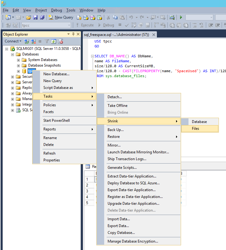
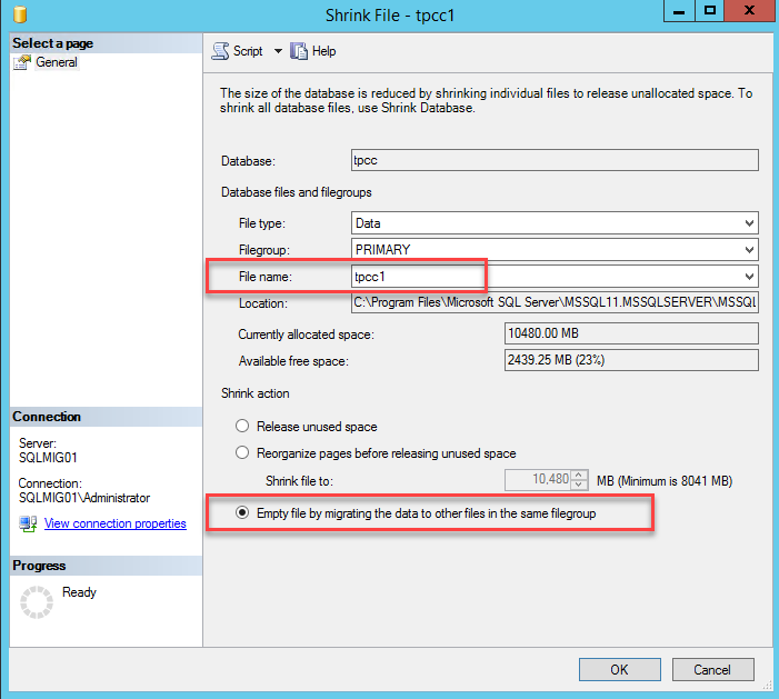
Now select the “Empty File by migrating data to other files in the same filegroup” option and press “Ok”.

Depending on the size of the database and the speed of the storage this may take some time and it will have at least some impact on the performance of the server. As such I recommend performing the process outside of peak hours if possible.

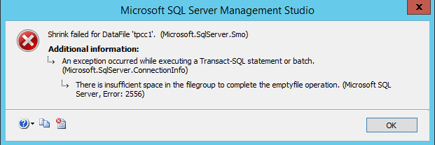
The error below is expected as we do not want to empty out the first *.mdf file completely. This is also an indication of our tasks being complete for empty file operation to the limit we’ve set earlier.

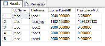
Once the task has completed you should see a roughly even distribution of data across the four database files by using the script below in query window.

USE tpcc
GO
SELECT DB_NAME() AS DbName,
name AS FileName,
size/128.0 AS CurrentSizeMB,
size/128.0 - CAST(FILEPROPERTY(name, 'SpaceUsed') 
AS INT)/128.0 AS FreeSpaceMB
FROM sys.database_files;

C:\Users\Kasim\AppData\Local\Temp\SNAGHTMLd751ece.PNG

Next we want to configure autogrow onto our databases so they can grow during business as usual operations.

The above shows the database are configured to autogrow by 100MB up to a limit of 2048MB each. The amount a database should autogrow will vary based on the rate of growth in your database, as will the file size limit so consider these values carefully.

Once you have set these settings it’s now time to shrink the original final to the same size as the other database files as shown below:

This process cleans up white space (empty space) within the database.

So far we have achieved the following:

  1. Updated the VM with additional PVSCSI controllers and more VMDKs
  2. Initialized the VMDKs and formatted to the Guest OS
  3. Created three new database files
  4. Balanced the database across the four database file (including the original file)

We have achieved all of this without taking the database offline.

At this stage the virtual machine and SQL can be left as is until such time as you can schedule a short maintenance window to perform the following:

  1. Copy the original DB file from C: to the remaining new database VMDK
  2. Copy the original Logs file from C: to the new logs VMDK

This process only takes a few minutes plus the time to copy the database and logs. The duration of the file copy will depend on the size of your database and the performance of the underlying storage. The good news is with the virtual machine having already been partially optimized with more PVSCSI controllers and VMDKs, the read (copy) process will be served by one SCSI controller/VMDK and the paste (write) process served by another which will minimize the downtime required.

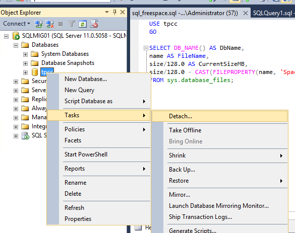
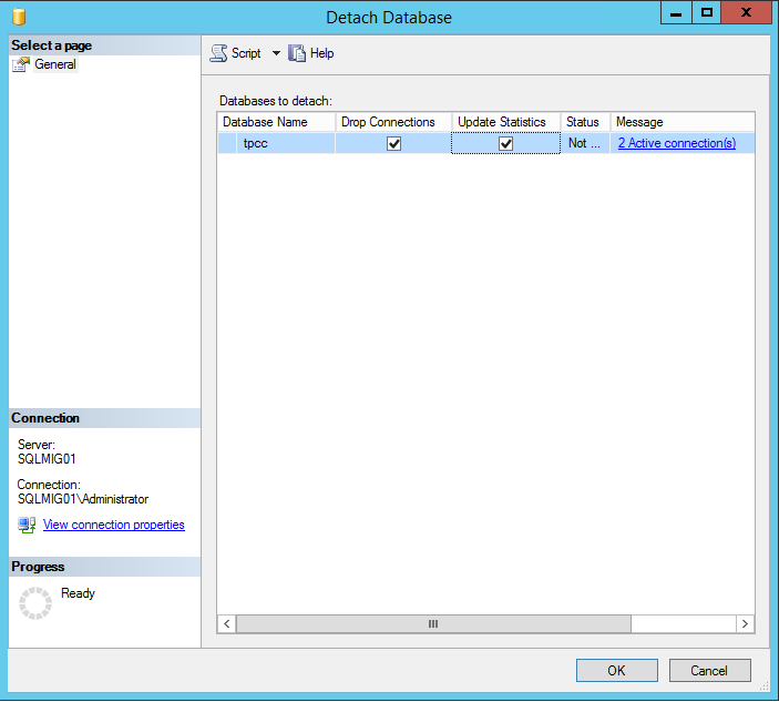
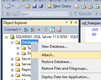
Once you have locked in your maintenance window, all you need to do is ensure all users and applications dependent on the database are shutdown, then detach the database and select the “Drop Connections” and “Update Statistics” and press Ok.


The next steps are very simple; we need to copy (or rather move/cut) the database from the original location as shown below:

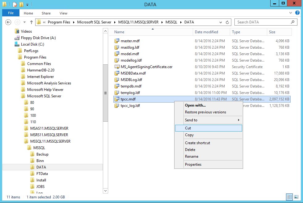
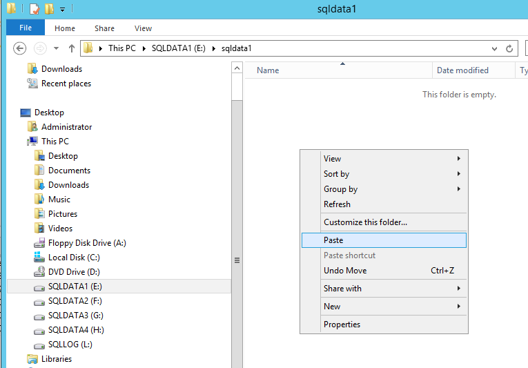
Now we paste the database file to the new data1 drive.

Then we copy the log file and paste it into the new log drive.

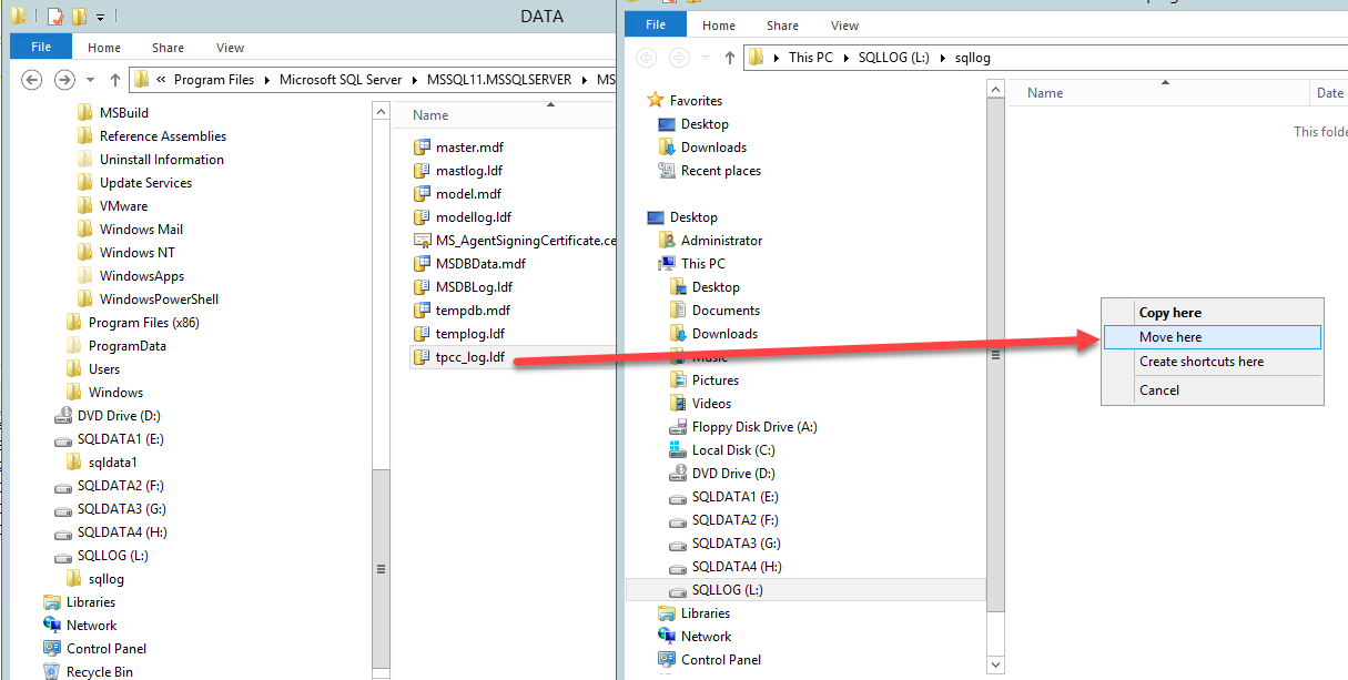
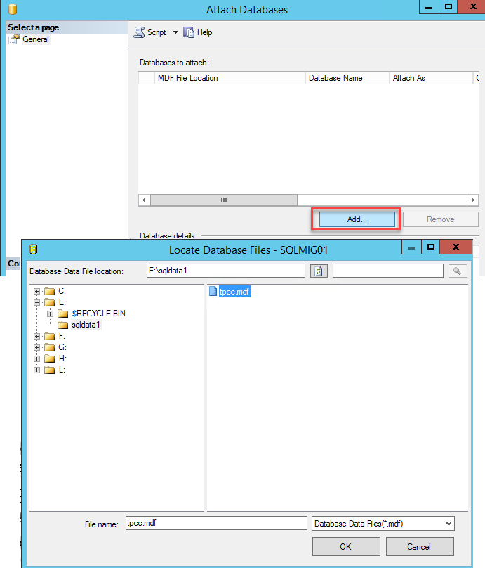
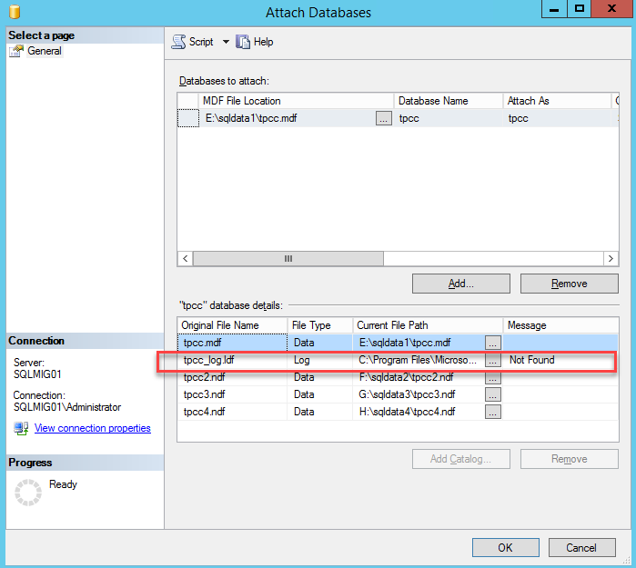
Now we simply reattach the database specifying the new location of the *.mdf file. You will note the message highlighted below which indicates the log files are not found which is expected since we have just relocated them.

C:\Users\Kasim\AppData\Local\Temp\SNAGHTMLd8094b4.PNG

To resolve this simply update the path to the logs file as shown below and press Ok.

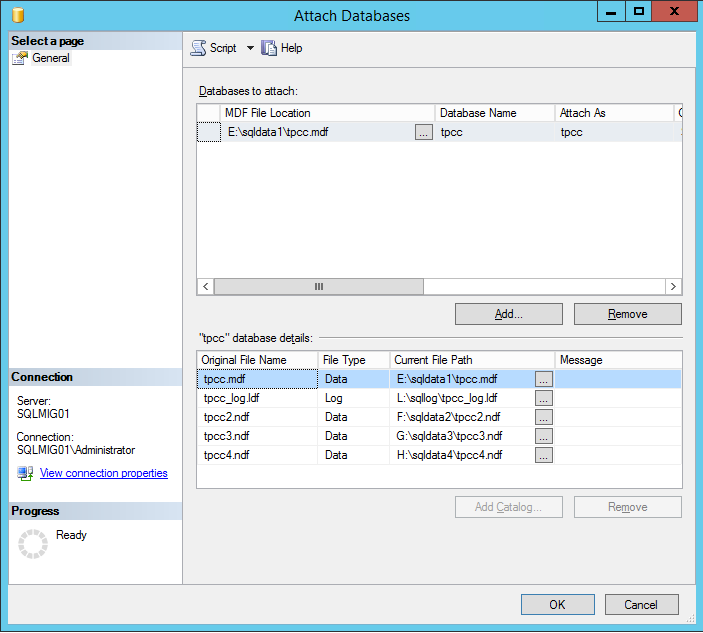
And we’re done! Simple as that.

Adjust the maximum growth of the datafile to an appropriate size. If you set to unlimited, please ensure that you monitor the volumes and manage them according to the growth rate of the database.

Lastly, don’t forget to change the database recovery model to Full

Now you have your OS separated from your SQL database and logs and all of the drives are configured across four virtual SCSI controllers.

Summary:

If you have an existing SQL server and storage performance is considered a problem, before buying new storage (Nutanix or otherwise), ensure you optimize the virtual machines storage layout as the constraint may not be the underlying storage.

As this post explains, most of this optimization can be done without taking the database offline so you don’t really have anything lose in following this process. Worst case scenario is performance does not improve and you have eliminated the VM storage as the constraining factor and when you do implement new Nutanix nodes or any underlying storage, you will get the most out of it. Do follow some other best practices like RAM to vCPU balancing, SQL Memory optimization, Trace Flags and database compression, be it row or page.

Acknowledgements:

A huge thank you to Kasim Hansia from the Nutanix Business Critical Applications (vBCA) team for documenting this process and allowing me to publish this post using his screenshots. It’s a pleasure working with such a talented group at Nutanix both in the vBCA team and in the broader organization.

Related Articles:

  1. SQL and Exchange performance in a virtual machine
  2. How to successfully virtualize Microsoft Exchange
  3. MS support for SQL on NFS datastores

SQL & Exchange performance in a Virtual Machine

The below is something I see far to often: An SQL or Exchange virtual machine using a single LSI Logic SAS virtual SCSI controller.

LSIlogic

What is even worse is a virtual machine using a single LSI controller and a single virtual disk for one or more databases and logs (as shown above).

Why is this so common?

Probably because the LSI Logic SAS controller is the default for Windows 2008/2012 virtual machines and additional SCSI controllers are not automatically added until you have more than 16 virtual disks for a single VM.

Why is this a problem?

The LSI controller has a queue depth limit of 128, compared to the default limit for PVSCSI which is 256, however it can be tuned to 1024 for higher performance requirements.

As a result, the a configuration with a single LSI controller and/or a limited number of virtual disks can artificially significantly constrain the underlying storage from delivering the performance it is capable of.

Another problem with the LSI controller is the amount of CPU it uses is higher than the PVSCSI controller for the same IO levels. This means you’re wasting virtual machine (and the underlying hosts) CPU resources unnecessarily.

Using more CPU could lead to other problems such as CPU Ready which can also lead to reduced performance.

A colleague and friend of mine, Michael Webster wrote a great post titled: Performance Issues Due To Virtual SCSI Device Queue Depths where he shows the performance difference between SATA, LSI and PVSCSI controllers. I highly recommend having a read of this post.

What is the solution?

Using multiple Paravirtual (PVSCSI) adapters with virtual disks evenly spread over the four controllers for Windows virtual machines is a no brainer!

This results in:

  1. Higher default queue depth
  2. Lower CPU overheads
  3. Higher potential performance

How do I configure this?

It’s fairly straight forward, but don’t just change the LSI Controller too PVSCSI as the Guest OS may not have the driver installed which will result in the VM failing to boot.

Too avoid this, simply edit the virtual machine and add a new Virtual Disk of any size and for the virtual device node, select SCSI (1:0) and follow the prompts.

VirtualDiskSCSI10

Once the new virtual disk is added you should see a new LSI Logic SAS SCSI controller is added as shown below.

NewLSIController

Next highlight the adapter and select “Change Type” in the top right hand corner of the window and select Paravirtual. Once this is complete you should see similar to the below:

AddPVSCSIController

Next hit “Ok” and the new Controller and virtual disk will be added to the VM.

Now we open the console of the VM and open Compute Management and goto Device Manager. Under Storage Controllers you should now see VMware PVSCSI Controller as shown below.

DeviceManagerPVSCSI

Now we are safe to Shutdown the VM.

Once the VM is shutdown, Edit the VM setting and highlight the SCSI Controller 0 and select Change Type as we did earlier and select Paravirtual. Once this is done you will see the original controller is replaced with a new controller.

ChangeLSItoPVSCSI

Now that we have the boot drive change to PVSCSI, we can now balance the data drives across up to four PVSCSI controllers for maximum performance.

To do this, simply highlight a Virtual Disk and drop down the Virtual Device Node and select SCSI (1:0) or any other available slot on the SCSI (1:x) controller.

ChangeControllerID

After doing this you will see new SCSI controllers appear and you need to change these to Paravirtual as we have done to the first controller.

ChangeControllerIDMultipleVdisks

For each of the virtual disks, ensure they are placed evenly across the PVSCSI controllers. For example, if you have a VM with eight virtual disks plus the OS disk, it should look like this:

Virtual Disk 1 (OS) : SCSI (0:0)
Virtual Disk 2 (OS) : SCSI (0:1)
Virtual Disk 3 (OS) : SCSI (1:0)
Virtual Disk 4 (OS) : SCSI (1:1)
Virtual Disk 5 (OS) : SCSI (2:0)
Virtual Disk 6 (OS) : SCSI (2:1)
Virtual Disk 7 (OS) : SCSI (3:0)
Virtual Disk 8 (OS) : SCSI (3:1)
Virtual Disk 9 (OS) : SCSI (0:2)

This results in two data virtual disks per PVSCSI controller which evenly distributes IO across all controllers with the exception being first controller (SCSI 0) also hosting the OS drive.

What if I have problems?

On occasions I have seen problems with this process which has resulted in VMs not booting, however these issues are easy to fix.

If your VM fails to boot with a message like “Operating System not found”, I suggest you panic! Just kidding, this is typically just the boot order of the Virtual machine has been screwed up. Just go into the bios and check the boot order has the PVSCSI controller showing and the correct virtual disk in first priority.

If the VM boots and BSOD or crashes and goes into a continuous reboot loop then power off the VM and set the first SCSI controller where the boot disk is running back to LSI. Then reboot the VM and make sure the PVSCSI driver is showing up (if its not you didn’t follow the above instructions) so go back and follow them so the PVSCSI driver is loaded and working, then shutdown and change the SCSI controller back to PVSCSI and you should be fine.

If the VM boots and one or more drives do not show up in my computer, go into Disk Manager and you may see the drives are marked as offline. Simply right click the drive and mark it as online and reboot and you’re good to go.

Summary:

If you have made the intelligent move to virtualize your business critical applications, firstly congratulations! However as with physical hardware, Virtual machines also have optimal configurations so make sure you use PVSCSI controllers with multiple virtual disks and have your DBA span the database across multiple virtual disks for maximum performance.

The following post shows how to do this in detail:

Splitting SQL datafiles across multiple VMDKs for optimal VM performance

If the DBA is not confident doing this, you can also just add multiple virtual disks (connected via multiple PVSCSI controllers) and create a stripe in guest (via Disk Manager) and this will also give you the benefit of multiple vdisks.

Related Articles:

1. Peak Performance vs Real World Performance

2. Enterprise Architecture & Avoiding tunnel vision

3. Microsoft Exchange 2013/2016 Jetstress Performance Testing on Nutanix Acropolis Hypervisor (AHV)

The All-Flash Array (AFA) is Obsolete!

Over the last few years, I’ve had numerous customers ask about how Nutanix can support bare metal workloads. Up until recently, I haven’t had an answer the customers have wanted to hear.

As a result, some customers have been stuck using their exisiting SAN or worse still being forced to go out and buy a new SAN.

As a result many customers who have wanted to use or have already deployed hyperconverged infrastructure (HCI) for all other workloads are stuck managing an all flash array silo to service some bare metal workloads.

In June at .NEXT 2016, Nutanix announced Acropolis Block Services (ABS) which now allows bare metal workloads to be serviced by new or existing Nutanix clusters.

ABSoverview

As Nutanix has both hybrid (SSD+SATA) and all-flash nodes, customers can chose the right node type/s for their workloads and present the storage externally for bare metal workloads while also supporting Virtual Machines and Acropolis File Services (AFS) and containers.

So why would anyone buy an all-flash array? Let’s discuss a few scenarios.

Scenario 1: Bare metal workloads

Firstly, what applications even need bare metal these days? This is an important question to ask yourself. Challenge the requirement for bare metal and see if the justifications are still valid and if so, has anything changed which would allow virtualization of the applications. But this is a topic for another post.

If a customer only needs new infrastructure for bare metal workloads, deploying Nutanix and ABS means they can start small and scale as required. This avoids one of the major pitfalls of having to size a monolithic centralised, dual controller storage array.

While some AFA vendors can/do allow for non-disruptive controller upgrades, it’s still not a very attractive proposition, nor is it quick or easy. and reduces resiliency during the process as one of two controllers are offline. Nutanix on the other hand performs one click rolling upgrades which mean the largest the cluster, the lower the impact of an upgrade as it is performed one node at a time without disruption and can also be done without risk of a subsequent failure taking storage offline.

If the environment will only ever be used for bare metal workloads, no problem. Acropolis Block Services offers all the advantages of an All Flash Array, with far superior flexibility, scalability and simplicity.

Advantages:

  1. Start small and scale granularly as required allowing customers to take advantage of newer CPU/RAM/Flash technologies more frequently
  2. Scale performance and capacity by adding node/s
  3. Scale capacity only with storage-only nodes (which come in all flash)
  4. Automatically scale multi-pathing as the cluster expands
  5. Solution can support future workloads including multiple hypervisors / VMs / file services & containers without creating a silo
  6. You can use Hybrid nodes to save cost while delivering All Flash performance for workloads which require it by using VM flash pinning which ensures all data is stored in flash and can be specified on a per disk basis.
  7. The same ability as an all flash array to only add compute nodes.

Disadvantages:

  1. Your all-flash array vendor reps will hound you.

Scenario 2: Mixed workloads inc VMs and bare metal

As with scenario 1, deploying Nutanix and ABS means customers can start small and scale as required. This again avoids the major pitfall of having to size a monolithic centralised, dual controller storage array and eliminates the need for separate environments.

Virtual machines can run on compute+storage nodes while bare metal workloads can have storage presented by all nodes within the cluster, including storage-only nodes. For those who are concerned about (potential but unlikely) noisy neighbour situations, specific nodes can also be specified while maintaining all the advantages of Nutanix one-click, non-disruptive upgrades.

Advantages:

  1. Start small and scale granularly as required allowing customers to take advantage of newer CPU/RAM/Flash technologies more frequently
  2. Scale performance and capacity by adding node/s
  3. Scale capacity only with storage-only nodes (which also come in all flash)
  4. Automatically scale multi-pathing for bare metal workloads as the cluster expands
  5. Solution can support future workloads including multiple Hypervisors / VMs / file services & containers without creating a silo.

Disadvantages:

  1. Your All-Flash array vendor reps will hound you.

What are the remaining advantages of using an all flash array?

In all seriousness, I can’t think of any but for fun let’s cover a few areas you can expect all-flash array vendors to argue.

Performance

Ah the age old appendage measuring contest. I have written about this topic many times, including in one of my most popular posts “Peak performances vs Real world performance“.

The fact is, every storage product has limits, even all-flash arrays and Nutanix. The major difference is that Nutanix limits are per cluster rather than per Dual Controller Pair, and Nutanix can continue to scale the number of nodes in a cluster and continue to increase performance. So if ultimate performance is actually required, Nutanix can continue to scale to meet any performance/capacity requirements.

In fact, with ABS the limit for performance is not even at the cluster layer as multiple clusters can provide storage to the same bare metal server/s while maintaining single pane of glass management through PRISM Central.

I recently completed some testing with where I demonstrated the performance advantage of storage only nodes for virtual machines as well as how storage-only nodes improve performance for bare metal servers using Acropolis Block Services which I will be publishing results for in the near future.

Data Reduction

Nutanix has had support for deduplication, compression for a long time and introduced Erasure Coding (EC-X) mid 2015. Each of these technologies are supported when using Acropolis Block Services (ABS).

As a result, when comparing data reduction with all-flash array vendors, while the implementation of these data reduction technologies varies between vendors, they all achieves similar data reduction ratios when applied to the same dataset.

Beware of some vendors who include things like backups in their deduplication or data reduction ratios, this is very misleading and most vendors have the same capabilities. For more information on this see: Deduplication ratios – What should be included in the reported ratio?

Cost

Here we should think about what are the age old problems are with centralized shared storage (like AFAs)? Things like choosing the right controllers and the fact when you add more capacity to the storage, you’re not (or at least rarely) scaling the controller/s at the same time come to mind immediately.

With Nutanix and Acropolis Block Services you can start your All Flash solution with three nodes which means a low capital expenditure (CAPEX) and then scale either linearly (with the same node types) or non-linearly (with mixed types or storage only nodes) as you need to without having to rip and replace (e.g.: SAN controller head swaps).

Starting small and scaling as required also allows you to take advantage of newer technologies such as newer Intel chipsets and NVMe/3D XPoint to get better value for your money.

Starting small and scaling as required also minimizes – if not eliminates – the risk of oversizing and avoids unnecessary operational expenses (OPEX) such as rack space, power, cooling. This also reduces supporting infrastructure requirements such as networking.

Summary:

As shown below, the Nutanix Acropolis Distributed Storage Fabric (ADSF) can support almost any workload from VDI to mixed server workloads, file, block , big data, business critical applications such as SAP / Oracle / Exchange / SQL and bare metal workloads without creating silos with point solutions.

NutanixSingleFabricAllWorkloads

In addition to supporting all these workloads, Nutanix ADSF scalability both from a capacity/performance and resiliency perspective ensures customers can start small and scale when required to meet their exact business needs without the guesswork.

With these capabilities, the All-Flash array is obsolete.

I encourage everyone to share (constructively) your thoughts in the comments section.

Note: You must sign in to comment using WordPress, Facebook, LinkedIn or Twitter as Anonymous comments will not be approved,

Related Articles:

  1. Things to consider when choosing infrastructure.

  2. Scale out performance testing with Nutanix Storage Only Nodes

  3. What’s .NEXT 2016 – Acropolis Block Services (ABS)

  4. Scale out performance testing of bare metal workloads on Acropolis Block Services (Coming soon)

  5. What’s .NEXT 2016 – Any node can be storage only

  6. What’s .NEXT 2016 – All Flash Everywhere!