Nutanix – Improving Resiliency of Large Clusters with Erasure Coding (EC-X)

As cluster sizes increase, it is important to understand the chance of multiple concurrent failure also increases and to architect solutions to ensure resiliency is maintained.

Because scalability is one of many strengths of the Nutanix Distributed Storage Fabric, Nutanix supported multiple data protection levels (RF2 and RF3) to ensure resiliency could be scaled with cluster size.

However using RF3 results in reducing the usable capacity to approximately 33% of the formatted capacity of the drives within the cluster which means it is sometimes considered undesirable.

But because some customers require the ability to support multiple concurrent node failures without the chance of data loss or unavailability, RF3 has been required.

Enter Nutanix Erasure Coding (EC-X)!

Now lets say you have a 32 node cluster where each node has 10TB RAW.

With RF3 we would have approx 3.33TB usable per node for a total of 106.56TB in the cluster.

With EC-X enabled (assuming EC-X has been applied to all data) the usable capacity would DOUBLE to 6.66TB per node and 213.12TB for the cluster.

Here’s how it works.

For RF3, the Nutanix Distributed Storage Fabric writes and maintains three copies of each piece of data. The below shows three copies of data “A” and “B”.

RF3

The below is a simplified example of what the Nutanix Distributed Storage Fabric looks like once EC-X is applied to RF3 data.

RF3plusECX

As you can see, we now support twice the amount of data as RF3 while still having dual parity. As a result, using RF3 + EC-X gives customers using large clusters MORE usable capacity than RF2 (~50% of RAW) while providing dual parity (which enables the loss of two nodes without data loss/unavailability).

Not bad for a software only upgrade!

So what do I recommend customers who are running 32 node or larger clusters?

1. For customers running RF3 already, Consider enabling EC-X.
2. For customers running RF2, consider enabling RF3 and EC-X

Nutanix – Erasure Coding (EC-X) Deep Dive

I published a post earlier this month during the .NEXT conference titled “What’s .NEXT? – Erasure Coding!” which covered the basics of Nutanix EC-X implementation.

This post is a deep drive follow on to answer numerous questions I have received about EC-X such as:

1. Does it work with Compression and De-duplication?
2. Can I use EC-X to reduce the overhead of RF3?
3. Does it work on Hot or Cold data?
4. Does it work only on the SATA tier?
5. What is the performance impact?
6. When should I use/not use EC-X?
7. What’s different about Nutanix (Patent pending) EC-X compared to other EC algorithms?
8. How does EC-X impact Data Locality?
9. What Hypervisors is EC-X supported with?

So let’s start with What’s different about Nutanix (Patent pending) EC-X compared to other EC algorithms?

* Nutanix EC-X is optimized for a distributed platform, where data is spread across nodes, not individual disks to ensure optimal performance. This also ensures rebuild times are faster and lower impact as the rebuild is performed across all the nodes/drives.

* Nutanix EC-X is also performed as a background task and only on Write Cold data meaning the configured RF is completed as normal and then as a post process EC-X is performed to ensure the write process is not potentially slowed by requiring numerous nodes within the cluster to participate in the initial write I/O.

How does EC-X affect existing Nutanix Data Reduction technologies.

* Short answer, EC-X is complimentary to both compression and deduplication so you will get even more data reduction. Here is a sample screen shot from the Home screen in PRISM which shows a breakdown of Dedup, Compression and Erasure Coding savings.

CapacityOptimization

In the Storage Tab within PRISM, we can get further details on the capacity savings. Here we see an example Container with Compression and EC-X enabled:

CompplusECXhighlighted

Does it work only on the SATA tier?

No, EC-X works on all tiers, being SSD and SATA today, but in the future when newer technology or more than two tiers are used, EC-X works across all tiers.

Does EC-X work on Hot or Cold data?

EC-X waits until data written (via RF2 or RF3) is “Write Cold”, meaning the data is not being overwritten. The data might be white hot from a read I/O perspective, but as long as its not being overwritten the extent group (4MB) will be a candidate for EC-X.

This means for data which is Write Cold, the effective capacity of the SSD tier will be increased due to requiring less space thanks to EC-X.

What is the performance impact?

As EC-X is a post process task and EC-X waits until data is “Write Cold” before performing EC-X on the data, in general it will not impact the Write performance.

The exception to this is in the event data is Write Cold for a period of time, then the data is overwritten, this “overwrite” will incur a higher penalty than a typical RF2/RF3 write. As such some workloads may not be suitable for EC-X which I will discuss later.

Overall, if the workload is suitable, EC-X will keep the data in the SSD tier and the parity on the SATA tier which effectively extends the usable capacity of the SSD tier therefore helping to increase performance (as with compression and dedup).

What Hypervisors is EC-X supported with?

Everything in the Nutanix Distributed Storage Fabric (part of the Nutanix Xtreme Computing Platform or XCP) is designed to be hypervisor agnostic. So whatever Hypervisor/s you choose, you can benefit from EC-X!

How does EC-X impact Data Locality?

As the initial Write path is not impacted by enabling EC-X, Data Locality is still maintained and ensures one copy of data is written to the local node where the VM is running while replicating a further one or two copies (dependent on RF configuration) throughout the cluster.

This means that for newly written data as well as data being overwritten at frequencies of <60mins will always maintain data locality.

For data which meets the criteria for EC-X to be performed, such as Read Hot or Write Cold data, Data Locality can only be partially maintained as the data is by design striped across nodes. The result of this means that it is probable Read I/O will be performed over the network.

Importantly though Read Hot data will be maintained in the SSD tier and be distributed throughout the cluster. This means a single VMs read I/O can be served by multiple nodes concurrently which can lead to increased performance.

As EC-X also provides capacity savings, this allows for more data to be serviced by the SSD tier which enabled a larger active working set to perform at SSD speeds.

In summary, while Data Locality is not always maintained when using EC-X, the advantages of EC-X far outweigh the partial loss in Data Locality.

And finally, When should I use/not use EC-X?

As discussed earlier, EC-X is applied to Write Cold data and if/when that data is overwritten, the write penalty is higher than a typical RF2 write I/O. So if your dataset has a high percentage of overwrites, it is recommended not to use EC-X. The good news is storage can be assigned on a per VMDK level (or vDisk at the NDFS layer) so you can have one VM using EC-X for some data and RF2/3 for other data, again giving customers the best of both worlds.

The best workloads for EC-X are:

1. File Servers
2. Backup
3. Archive
4. Email
5. Logging

Summary:

Nutanix EC-X gives customers more choice without compromising functionality and performance while dramatically reduces the cost/GB of storage.

Related Articles:

  1. Large scale clusters and increased resiliency with RF3 + EC-X
  2. What I/O will Nutanix Erasure coding (EC-X) take effect on?

  3. Sizing assumptions for solutions with Erasure Coding (EC-X)

Calculating Actual Usable capacity? It’s not as simple as you might think! – Part 2 Nutanix

In Part 1, the example provided showed usable capacity for a SAN/NAS using a combination of RAID 10, RAID 5 and RAID 6 along with the various sizing considerations resulted in 35.68TB usable capacity or approx 1/3rd of the RAW 100TB.

In Part 2 we will discuss the misconception that Nutanix (a Hyper-converged platform) provides lower effective usable capacity compared to SAN or NAS solutions.

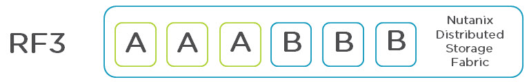
At a high level, Nutanix uses Replication Factor 2 (RF2) which has the same overhead as RAID 1 so straight away a lot of people jump to the conclusion that the usable capacity is less that a traditional SAN/NAS because *insert your favourite RAID level here* has less overhead.

Let’s say we have a Nutanix cluster with 100TB Raw storage using the most common node type, the NX3050.

Now let’s address the same points as we did in Part 1 for the SAN/NAS example:

So starting with the same 100TB RAW as we did for the SAN/NAS example and see where things end up on Nutanix.

1. Deducting hot spare drives

Nutanix does not use hot spare drives, data is balanced across all drives in the “Storage Pool”. To cater for failure, it is recommended to size for N+1 for Resiliency Factor 2 (RF2) deployments. If we we’re using NX3050 nodes (the most popular Nutanix node) then the overhead of N+1 would be ~4.8TB RAW.

100TB – N+1 Node (4.8TB RAW) = 95.2TB

2. RAID Overhead

Nutanix doesn’t use RAID, but the Replication Factor 2 has an overhead is 50% (the same as RAID10).

95.2TB – 50% (RF2) = 47.6TB remaining

3. Free Space on the platform required to ensure performance

For Nutanix all write I/O goes to either the Extent Storage or Oplog, both of which are housed on the SSD tier. All random writes are serviced by the Oplog until it reaches 95% capacity at which point the oplog is bypassed.

As such, performance remains high until 95% capacity. Therefore only 5% free capacity is required to ensure high performance.

47.6TB – 5% (Free space for performance) = 45.2TB

FYI: Nutanix Performance and Engineering team members including myself typically conduct benchmarks at greater than 90% cluster capacity.

4. Free space per LUN

Nutanix does not use LUNs. Nutanix presents containers to the hypervisor. All containers are thin provisioned and all containers can use all available space in the storage pool. Meaning free space only needs to be managed at the Storage Pool layer, not at each individual container.

As we have already taken into account the 5% free space there is no need to take another 5% of space therefore we remain at 45.2TB usable.

5. Free space per VMDK

As with physical servers and SAN/NAS environments, we don’t want our VMs drives running out of capacity, as a result it is common to size VMDKs well above what is strictly required to make capacity management (operational tasks) easier.

As mentioned in Part 1, I typically see architects recommending upwards of 10-20% free space per VMDK over and above what is required to account for unexpected growth, OS patching etc. This makes perfect sense for the same reason as we have free space per LUN because if space runs out for a VM, it’s another bad day for I.T.

For this example, I will assume the same 10% free space per VMDK as I did for SAN/NAS example, the difference with Nutanix is performance remains the same regardless of the VMDK being Thick or Thin provisioned, so with every VM Thin Provisioned, no capacity is required to be reserved for free space within VMDK files as it would be for traditional environments requiring Eager Zero Thick VMDKs for performance..

So we’re still at 45.2TB usable.

Now where are we at?

So far, the first 5 points are fairly easy to calculate.

Next we will look at various factors which further reduce usable capacity for SAN/NAS and see how they apply to Nutanix.

6. Silos for Performance

Nutanix does not require nor recommend silos being created for performance reasons. All VMs can reside in a single container therefore no capacity is unusable as a result of performance requirements.

As no silos are required for maximum performance, we are still at 45.2TB usable.

7. Silos of (or Fragmented) Usable Capacity

Nutanix does not configure usable capacity to containers, a container can use all the available storage in the underlying Storage Pool. Where multiple containers are provisioned, each container can see the total capacity of the storage pool while providing logical separation of the VMs within the containers. This avoids the issue of fragmented free capacity.

The diagram below shows 5 containers hosted by an example Nutanix cluster (Storage Pool) with 100TB total capacity, each container has a capacity of 100TB and 25TB free space in alignment with the underlying storage pool.

NutanixFreeSpace

In this case, when creating a new VM, or adding or expanding VMDKs for existing VMs, it does not matter which container we place the VM, as long as it is less than the 25TB available in the pool, it makes no difference to capacity.

This removes the requirement for complex capacity management, or using Storage DRS and Storage vMotion.

So we’re still at 45.2TB usable.

Other factors which reduce usable capacity?

8. LUN Provisioning Type

In many cases, especially when talking about high performance applications, storage vendors recommend using Thick Provisioned LUNs and as mentioned in Part 1, It’s anyone’s guess how much space is wasted as a result.

But with Nutanix, all containers are Thin Provisioned so no capacity is wasted on Thick Provisioning and performance is optimal

9. Wasted Capacity from using SSDs as Cache

Nutanix does not use SSDs as Cache! The SSD’s form part of the Extent Store which is for persistent data storage. The OpLog which is also on SSD is also persistent and not a “cache”. As such, no capacity is being reduced as a result of caching.

10. Snapshot Reserves

Nutanix does not use reserve capacity for snapshots. Snapshots simply use available capacity in the storage pool. If you don’t use snapshots, no space is wasted, if you do use snapshots, then the delta changes are stored. Simple as that.

Summary:

From the 100TB RAW factoring in what is a realistic Nutanix configuration including N+1 to tolerate a node failure and support the cluster being able to fully self heal the effective usable capacity is 45.2TB which is just under 50% of 100TB RAW.

This is a very simple configuration to manage from both a performance and capacity perspective, and one which is easily calculated and repeatable.

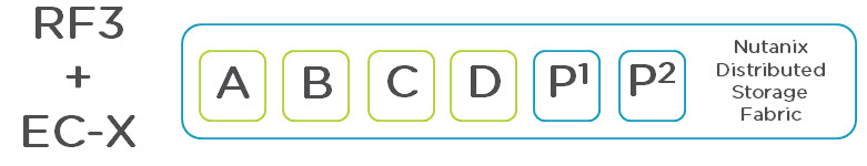
If the Resiliency Factor was 3 (which IMO is rarely if ever required) across the entire environment (which again would be extremely unusual as VMs which require RF3 can be configured in an RF3 container) then the usable capacity would be ~30TB which is only sightly below the SAN/NAS example and RF3 delivers higher resiliency.

In reality, >95% of workloads should be deployed on RF2, with a very small number of VMs possibly using RF3. In reality RF2 is extremely resilient and self healing so IMO RF3 is rarely required.

So in conclusion, Nutanix usable capacity is ~50% of RAW capacity, the difference between Nutanix and traditional SAN/NAS is you actually can use almost all the “usable” capacity and maintain optimal performance with little/no complexity.

Nutanix also has data reduction technologies such as Compression and De-duplication, along with intelligent cloning to increase the effective capacity of the storage pool.

While I believe Nutanix’ usable capacity today is excellent especially when considering how resilient RF2 is and comparing usable capacity to many products on the market, Nutanix has the advantage of not being constrained by legacy technologies such as RAID, so I’ll leave you with a little teaser:

Usable capacity will be improving significantly in upcoming releases of Nutanix Operating System. 🙂