Nutanix X-Ray Benchmarking tool – Introduction

I’ve been excited to write about X-ray for a while now, but I’ve not had the time. But the opportunity has presented itself where I could kill two birds with one stone and do some performance comparisons between Nutanix AHV Turbo Mode and other platforms on the same underlying hardware, so what better time to review X-ray as part of this process.

So for those of you who have not heard of X-Ray, it wouldn’t be unreasonable to assume it’s just another benchmarking tool to further muddy the waters when comparing different platforms.

However X-Ray takes a different approach, to quote Paul Updike who is part of Nutanix Technical Marketing Engineering:

Normally performance is your test variable and you measure the effect on the system. X-ray is upside down, performance of an app in a VM is the control and our test variable is the system. We measure the effect on the control.

So if all you want is “hero numbers” you’ve come to the wrong place, although  X-Ray does have a peak performance micro-benchmark test built-in, it’s far from real world in comparison to the other tests within X-ray.

The X-Ray virtual appliance is recommended to be ran on a cluster which is not the target for the testing, such as a management cluster. But for those environments where this additional hardware may not be available, it can also be deployed on VirtualBox or VMware Workstation on your PC or laptop.

Also if you have an Intel NUC, you could deploy Nutanix Community Edition (CE) and run X-Ray on CE which is based on AHV.

In addition to the different approach X-ray takes to benchmarking, I like that X-ray performs fully automated testing across multiple hypervisors including ESXi, AHV as well as different underlying storage. This helps ensure consistent and fair comparisons between platforms, or even comparisons between Nutanix node types if you decide to compare model types before making a purchasing decision.

X-ray has several built in tests which are focused not just on outright performance, but on how a system functions and performs during node failure/s, with snapshots as well as during rolling upgrades.

The reason Nutanix took this approach is because it is much more real world than simply firing up I/O meter with lots of outstanding I/O with a 100% random 4k read. In the real world, customers performance upgrades (hopefully regularly to take advantage of new functionality and performance!), hardware does fail when we can least afford it and using space efficient snapshots as part of an overall backup strategy makes a lot of sense.

Now let’s take a look at the X-Ray interface starting with an overview:

XrayOverview

X-Ray is designed to be similar to PRISM to keep that great Nutanix look and feel. The tool is very simple to use with three sections being Tests, Analyses and Targets.

To get started is very quick/easy, just open the “Targets” view (shown below) and select “New Target”.

XrayTargets

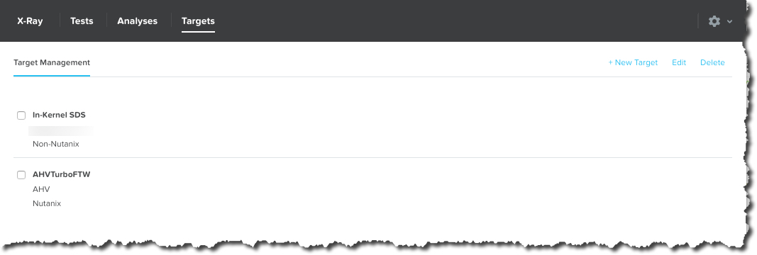
In the “Create Target” popup, you simply, provide a name for the target e.g.: “Nutanix NX-3460 Cluster AHV”, select the Manager type, being either vCenter for ESXi environments or PRISM for AHV.

Then select the cluster type, being Nutanix (i.e.: A Nutanix NX, Dell XC, Lenovo HX or HPE/Cisco software only) OR “Non-Nutanix” which is for comparisons with platforms not running Nutanix AOS such as VMware vSAN.

XrayCreateTarget

For VMware environments, you then provide the vCenter details and regardless of the hardware type or platform, you supply the out of band management (e.g.: IPMI) details. The out of band management details allow X-ray to perform simulated hardware failure tests which are critical to any product evaluation and pre-production operational verification testing.

X-Ray then allows you to select the cluster, container (or datastore) and networking (e.g.: Port Group) to be used for the testing.

XrayCreateTarget_Cluster

X-ray then discovers the nodes (e.g.: ESXi Hosts) and allows you to add nodes and confirm the IPMI type to ensure maximum compatibility.

XrayCreateTarget_Node

Now hit “Save” and you’re good to go! Pretty simple right?

Now to run a test, simply click the test you want to run and select “Add to Queue”.

Xray_RunTestVDISim

The beauty of this is X-ray allows you to queue as many tests as you want and leave the system to run the tests, say overnight or over a weekend without requiring you to monitor them and start tests one by one.

In between tests the target systems are cleaned up (i.e.: data and VMs deleted) to ensure consistent / fair results even when running test packages one after another.

Once a test has been ran, you can view the results in the X-Ray GUI (as shown below):

XrayTestsOverview

You can also generate a PDF report for individual tests or perform analysis between two tests including of different platforms:

XrayAnalyses

The above results show and overlay between two platforms, the first being AHV (although it’s incorrectly named Turbo mode when it was ran using non Turbo mode AOS version 5.1.1). As we can see, AHV even without turbo mode was more consistent than the other platform.

To create a PDF report, simply use the “Actions” drop down menu and select “Create Report”.XrayCreateReport

The report will create a report which covers off details about X-ray, the Target cluster/s, the scenario being tested and the test results.

XrayTOCReport

It will show simple results such as if the test passed (i.e.: Completed the required tasks) and things like test duration as shown below:

XrayReportTargetOverview

X-Ray also provides built-in tests for mixed workloads, which is much more realistic than testing peak performance for point (or siloed) solutions which are become more and more rare these days. XrayMixedWorkloads

X-Ray’s built in tests are also auto scaling based on the cluster size of the target and allow tuning of the scenario. For example, in the VDI simulator scenario, Task, Knowledge or Power Users can be selected.

XRayVDISimulator
Summary:

X-Ray provides a tool which is free of charge, multi-hypervisor, multi-platform (including non-HCI) which is easy to use for proof of concepts, product comparisons as well as real world, operational verification.

I am working with the X-ray team to develop new built in test scenarios to simulate real world scenarios for business critical applications as well as to allow customers and 3rd parties to validate the benefits of functionality such as data locality.

The following is a series of posts covering Nutanix AHV Turbo Mode performance/functionality comparisons with other products.

Nutanix X-Ray Benchmarking tool Part 2 -Snapshot Impact Scenario

Nutanix X-Ray Benchmarking tool Part 3 – Extended Node Failure Scenario

The truth about storage benchmarking

Recently I was asked to review some performance testing done by an external party and my initial impression was the performance was well below what I expected.

So over the weekend I setup a block in my lab to reproduce the tests to see if the results were firstly repeatable, and if so, what performance would I get with and without tuning.

The only significant difference between my hardware and the hardware used by the 3rd party was that I used old dual socket Ivy Bridge E5-2670 2.6Ghz 8c processors and the 3rd party had a much newer dual Broadwell E5-2640 v4 2.4Ghz processors.

If we compare the two processors using CPUBoss.com we see the following:

CPUboss1

Not surprisingly the Broadwell E5-2640 v4 processor is faster, but possibly less than you would expect with a 16.28% better PassMark per core, and in my opinion, the per core value quite importaint especially when considering business critical applications.

None the less, a 16.28% performance improvement per core will be a significant factor for a benchmark with Nutanix as the Controller VM (CVM) is powered by the CPU of the host.

I thought I would whip up a quick post about performance benchmarking to show how different performance results can be on the same hardware depending on just a few factors and why storage benchmarking, especially competitive benchmarking, cannot and should not be trusted when making purchasing decisions.

This test was for a 10k user MS Exchange deployment and the hardware used for testing was performed on in both cases was 1 x 1.92TB SSD and 3 x 4TB SATA drives and they were both tested on the same GA Nutanix AOS build.

The required (or Target) IOPS was just 216 per MS Exchange instance (VM) as shown below by the Jetstress report.

TargetIO

This target is calculated by Jetstress when using the “Exchange Mailbox Profile” test scenario with the following configuration:

MailboxProfile2

The resulting SSD vs SATA ratio makes this test largely about the limitations of SATA performance as >87% of data is being read from the SATA tier.

TierUsage

Test 1: The Jetstress dataset was created and then the performance test was immediately ran for 2hrs with no pre-warming of the metadata or read cache.

Achieved Transactional I/O: 200.663
Avg Log Write Latency: 1.06ms
Avg DB Write Latency: 1.4ms
Avg DB Read Latency: 14ms

This result was 15.61% lower than the 3rd parties result and interestingly if we correct for CPU core performance, it’s less than 1% difference. As this was in line with my expectation knowing the importance of CPU clock speed, I would say for this testing that the baseline results were comparable.

Test 2: The Nutanix tiering was tuned to suit large working sets (which vastly exceed the SSD tier) and the Jetstress dataset was created and the performance test was immediately ran for 2hrs again with no pre-warming of the metadata or read cache.

Before we get to the results, I want to point out that Jetstress is in some ways is very good but in other ways a very unrealistic benchmarking tool as the entire dataset is “active” which is not the case in the real world. However, in one way this is a good thing because a passing Jetstress result in my experience means the production deployment performs very well from a storage perspective especially when using tiered storage which is built around the assumption not all data is active. As a result, a Jetstress test could be considered a “worse case scenario” style test for intelligent tiered storage.

Achieved Transactional I/O: 249.623
Avg Log Write Latency: 0.99ms
Avg DB Write Latency: 1.5ms
Avg DB Read Latency: 12ms

Test 3: I then setup Jetstress as per Nutanix MS Exchange best practices and ran the test again with no pre-warming of the metadata or read cache.

Achieved Transactional I/O: 389.753
Avg Log Write Latency: 0.95ms
Avg DB Write Latency: 2.0ms
Avg DB Read Latency: 17ms

Test 4: I then lowered the Jetstress thread count to the lowest value (roughly 33% lower) which I estimated would achieve the target IOPS (this is to simulate real world requirements) and ran the test again with no pre-warming of the metadata or read cache.

Achieved Transactional I/O: 300.254
Avg Log Write Latency: 0.94ms
Avg DB Write Latency: 1.5ms
Avg DB Read Latency: 12ms

Note: Test 4 achieved the highest I/O per thread.

Test 5: The same configuration as Test 4 but with pre-warming of the metadata cache.

Achieved Transactional I/O: 334
Avg Log Write Latency: 0.98ms
Avg DB Write Latency: 1.9ms
Avg DB Read Latency: 12.4ms

Some of you might be asking, how did test 4 achieve higher transactional I/O and with lower read and write latency than Test 1 & 2 with less threads. Shouldn’t a higher thread count achieve higher IOPS?

The reasons is because the original thread count was pushing the SATA drives past their capabilities, leading to excessive latency. Lowering the thread count allowed the SATA drives to operate at somewhere around their most efficiency range leading to lower latency.

Test 6: The same configuration as Test 5 but with tuned extent cache (RAM read cache) and 100% medadata cached.

Achieved Transactional I/O: 362.729ms
Avg Log Write Latency: 0.92ms
Avg DB Write Latency: 1.7ms
Avg DB Read Latency: 12ms

As we can see from Test 1 through to Test 6, the performance differs by up to 81% depending on how the platform is configured.

Side note and future looking statement. Many of the optimisations I performed above wont be required for long as many of the areas these optimisations help improve are being addressed in upcoming code. In saying that, for a business critical application like Exchange, I don’t think it’s a problem doing some optimisation as long as 90% of the workloads run well by default and we’re only tuning for the 10% (vBCA) workloads.

But out of interest, what would happen if we enabled data reduction? How much of a performance hit would that take?

Test 7: The same configuration as Test 6 but with In-line compression enabled.

Achieved Transactional I/O: 751.275
Avg Log Write Latency: 0.97ms
Avg DB Write Latency: 3.4ms
Avg DB Read Latency: 5.9ms

That’s a 107.46% increase in transactional IO and with in-line compression! Log write latency remained sub ms and read latency has almost halved.

Note: As Jetstress data is highly compressible, (Nutanix achieves 8:1 or higher with non default settings), I tuned the compression slice size to give a more realistic data reduction ratio. The ratio for this test was 3.99:1 and the ratio of SSD to SATA was almost exactly 50% as shown below.

TierUsageAfterCompression

Why did performance improve so much with In-Line compression? Well there is two main reasons:

  1. More data is being served from the SSD tier as compression allows more effective SSD tier capacity.
  2. Reads from SATA are faster as less physical data needs to be read to service an I/O due to it being compressed. The higher the compression ratio, the more this can improve.

As we can see, the results varied significantly and had I wanted to optimise the test further, I could have achieved even higher performance but there was no need. The requirements for the solution were already achieved and in the case of Test 7, the requirements were exceeded by 247% meaning the solution had heaps of headroom.

Nutanix best practice is to enable In-line compression for MS Exchange and other databases such as Oracle and SQL as per my tweet below.

This testing was performed on Nutanix Acropolis Hypervisor (AHV) but was not using the upcoming Turbo mode, which will further improve performance and lower overheads.

This is a key point many people forget when benchmarking. If we assume the platforms in question are scalable (e.g.: Like Nutanix), it doesn’t matter if one platform does 100k IOPS and another does 200k IOPS if your requirements are 20k IOPS. Both platforms capabilities vastly exceed the requirement (10k IOPS) from a performance perspective, so performance is not longer a significant factor in your purchasing decision.

Question: Are the above performance results genuine?

All of the above results could be argued to be genuine results, at the same time none of the above represent the best performance that could be achieved, yet the results could be used to try and create FUD if they are improperly represented (which is almost always the case with competitive comparisons whether intentional or otherwise).

Let’s say this was your proof of concept, What should be the take away from benchmarking results like this?

Simple: The solution meets/exceeds your performance requirements.

Now for the point of this article: The truth about storage benchmarking is that there are so many variables that can affect the results that unless you’re truely experienced in benchmarking your applications AND an expert in the platforms you’re benchmarking, your results are unlikely to be indicative of the platforms capabilities and therefore of very little value.

If you’re benchmarking Vendor A vs Vendor B, it’s a waste of time doing “Like for Like” benchmarking because the Virtual machine and application settings which are optimal for one vendor, will likely be different for the other vendor. e.g.: SAN vs HCI.

On the other hand, a more valid test would be vendor A’s best practices vs vendor B best practices, but again if one vendor Jetstress achieves 500 and the other achieves 400, that 20% higher performance is all but irrelevant if your requirements are say, 216 like in this case.

A very good example of invalid “like for like” benchmarking would be to size the active working set (i.e.: The capacity of the data you plan to benchmark against) to fit within the cache/SSD tier of one platform, but exceed the cache/SSD capacity of the other platform. The results will be vastly different and will not be indicative of real world performance. This is what vendors do when competitive benchmarking and it’s likely one of the main reasons we see End User License Agreements (EULA) from most if not all storage vendors preventing publishing benchmark results without written agreement.

So the (unpopular) truth about storage benchmarking is it’s not as easy and building a VM and running I/O meter with the same profile on multiple system like some vendors and even 3rd party storage analysts would have you believe. The vast majority of people (customers, analysts and even vendors) doing benchmarking don’t have the skill/experience to produce repeatable or meaningful results, especially on multiple platforms.

In fact it’s unrealistic/unreasonable to expect a person (customer, vendor, consultant) to be an expert in multiple platforms, and very few people are!

Related Articles:

  1. Peak Performance vs Real World Performance
  2. The Key to performance is Consistency

SQL & Exchange performance in a Virtual Machine

The below is something I see far to often: An SQL or Exchange virtual machine using a single LSI Logic SAS virtual SCSI controller.

LSIlogic

What is even worse is a virtual machine using a single LSI controller and a single virtual disk for one or more databases and logs (as shown above).

Why is this so common?

Probably because the LSI Logic SAS controller is the default for Windows 2008/2012 virtual machines and additional SCSI controllers are not automatically added until you have more than 16 virtual disks for a single VM.

Why is this a problem?

The LSI controller has a queue depth limit of 128, compared to the default limit for PVSCSI which is 256, however it can be tuned to 1024 for higher performance requirements.

As a result, the a configuration with a single LSI controller and/or a limited number of virtual disks can artificially significantly constrain the underlying storage from delivering the performance it is capable of.

Another problem with the LSI controller is the amount of CPU it uses is higher than the PVSCSI controller for the same IO levels. This means you’re wasting virtual machine (and the underlying hosts) CPU resources unnecessarily.

Using more CPU could lead to other problems such as CPU Ready which can also lead to reduced performance.

A colleague and friend of mine, Michael Webster wrote a great post titled: Performance Issues Due To Virtual SCSI Device Queue Depths where he shows the performance difference between SATA, LSI and PVSCSI controllers. I highly recommend having a read of this post.

What is the solution?

Using multiple Paravirtual (PVSCSI) adapters with virtual disks evenly spread over the four controllers for Windows virtual machines is a no brainer!

This results in:

  1. Higher default queue depth
  2. Lower CPU overheads
  3. Higher potential performance

How do I configure this?

It’s fairly straight forward, but don’t just change the LSI Controller too PVSCSI as the Guest OS may not have the driver installed which will result in the VM failing to boot.

Too avoid this, simply edit the virtual machine and add a new Virtual Disk of any size and for the virtual device node, select SCSI (1:0) and follow the prompts.

VirtualDiskSCSI10

Once the new virtual disk is added you should see a new LSI Logic SAS SCSI controller is added as shown below.

NewLSIController

Next highlight the adapter and select “Change Type” in the top right hand corner of the window and select Paravirtual. Once this is complete you should see similar to the below:

AddPVSCSIController

Next hit “Ok” and the new Controller and virtual disk will be added to the VM.

Now we open the console of the VM and open Compute Management and goto Device Manager. Under Storage Controllers you should now see VMware PVSCSI Controller as shown below.

DeviceManagerPVSCSI

Now we are safe to Shutdown the VM.

Once the VM is shutdown, Edit the VM setting and highlight the SCSI Controller 0 and select Change Type as we did earlier and select Paravirtual. Once this is done you will see the original controller is replaced with a new controller.

ChangeLSItoPVSCSI

Now that we have the boot drive change to PVSCSI, we can now balance the data drives across up to four PVSCSI controllers for maximum performance.

To do this, simply highlight a Virtual Disk and drop down the Virtual Device Node and select SCSI (1:0) or any other available slot on the SCSI (1:x) controller.

ChangeControllerID

After doing this you will see new SCSI controllers appear and you need to change these to Paravirtual as we have done to the first controller.

ChangeControllerIDMultipleVdisks

For each of the virtual disks, ensure they are placed evenly across the PVSCSI controllers. For example, if you have a VM with eight virtual disks plus the OS disk, it should look like this:

Virtual Disk 1 (OS) : SCSI (0:0)
Virtual Disk 2 (OS) : SCSI (0:1)
Virtual Disk 3 (OS) : SCSI (1:0)
Virtual Disk 4 (OS) : SCSI (1:1)
Virtual Disk 5 (OS) : SCSI (2:0)
Virtual Disk 6 (OS) : SCSI (2:1)
Virtual Disk 7 (OS) : SCSI (3:0)
Virtual Disk 8 (OS) : SCSI (3:1)
Virtual Disk 9 (OS) : SCSI (0:2)

This results in two data virtual disks per PVSCSI controller which evenly distributes IO across all controllers with the exception being first controller (SCSI 0) also hosting the OS drive.

What if I have problems?

On occasions I have seen problems with this process which has resulted in VMs not booting, however these issues are easy to fix.

If your VM fails to boot with a message like “Operating System not found”, I suggest you panic! Just kidding, this is typically just the boot order of the Virtual machine has been screwed up. Just go into the bios and check the boot order has the PVSCSI controller showing and the correct virtual disk in first priority.

If the VM boots and BSOD or crashes and goes into a continuous reboot loop then power off the VM and set the first SCSI controller where the boot disk is running back to LSI. Then reboot the VM and make sure the PVSCSI driver is showing up (if its not you didn’t follow the above instructions) so go back and follow them so the PVSCSI driver is loaded and working, then shutdown and change the SCSI controller back to PVSCSI and you should be fine.

If the VM boots and one or more drives do not show up in my computer, go into Disk Manager and you may see the drives are marked as offline. Simply right click the drive and mark it as online and reboot and you’re good to go.

Summary:

If you have made the intelligent move to virtualize your business critical applications, firstly congratulations! However as with physical hardware, Virtual machines also have optimal configurations so make sure you use PVSCSI controllers with multiple virtual disks and have your DBA span the database across multiple virtual disks for maximum performance.

The following post shows how to do this in detail:

Splitting SQL datafiles across multiple VMDKs for optimal VM performance

If the DBA is not confident doing this, you can also just add multiple virtual disks (connected via multiple PVSCSI controllers) and create a stripe in guest (via Disk Manager) and this will also give you the benefit of multiple vdisks.

Related Articles:

1. Peak Performance vs Real World Performance

2. Enterprise Architecture & Avoiding tunnel vision

3. Microsoft Exchange 2013/2016 Jetstress Performance Testing on Nutanix Acropolis Hypervisor (AHV)