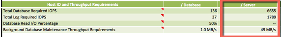
The below is something I see far to often: An SQL or Exchange virtual machine using a single LSI Logic SAS virtual SCSI controller.
What is even worse is a virtual machine using a single LSI controller and a single virtual disk for one or more databases and logs (as shown above).
Why is this so common?
Probably because the LSI Logic SAS controller is the default for Windows 2008/2012 virtual machines and additional SCSI controllers are not automatically added until you have more than 16 virtual disks for a single VM.
Why is this a problem?
The LSI controller has a queue depth limit of 128, compared to the default limit for PVSCSI which is 256, however it can be tuned to 1024 for higher performance requirements.
As a result, the a configuration with a single LSI controller and/or a limited number of virtual disks can artificially significantly constrain the underlying storage from delivering the performance it is capable of.
Another problem with the LSI controller is the amount of CPU it uses is higher than the PVSCSI controller for the same IO levels. This means you’re wasting virtual machine (and the underlying hosts) CPU resources unnecessarily.
Using more CPU could lead to other problems such as CPU Ready which can also lead to reduced performance.
A colleague and friend of mine, Michael Webster wrote a great post titled: Performance Issues Due To Virtual SCSI Device Queue Depths where he shows the performance difference between SATA, LSI and PVSCSI controllers. I highly recommend having a read of this post.
What is the solution?
Using multiple Paravirtual (PVSCSI) adapters with virtual disks evenly spread over the four controllers for Windows virtual machines is a no brainer!
This results in:
- Higher default queue depth
- Lower CPU overheads
- Higher potential performance
How do I configure this?
It’s fairly straight forward, but don’t just change the LSI Controller too PVSCSI as the Guest OS may not have the driver installed which will result in the VM failing to boot.
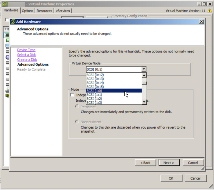
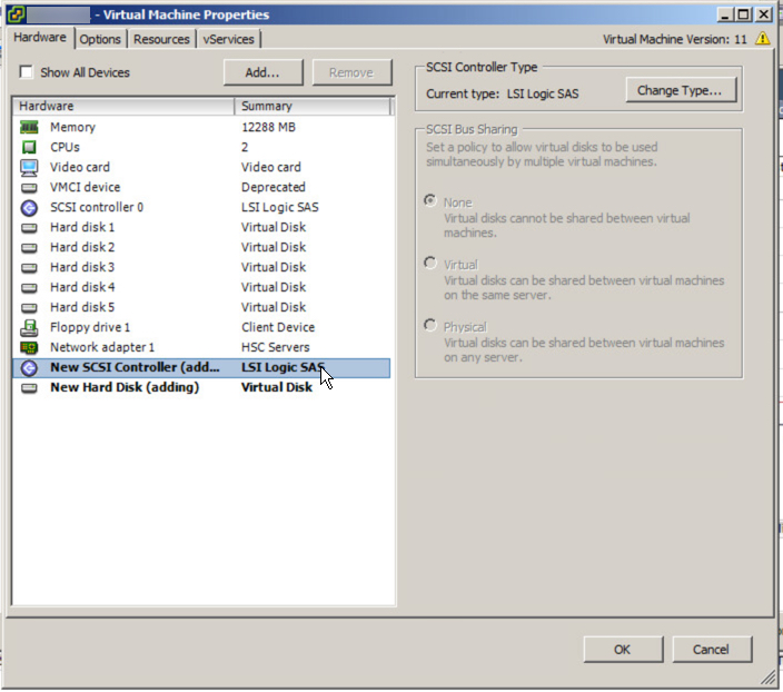
Too avoid this, simply edit the virtual machine and add a new Virtual Disk of any size and for the virtual device node, select SCSI (1:0) and follow the prompts.
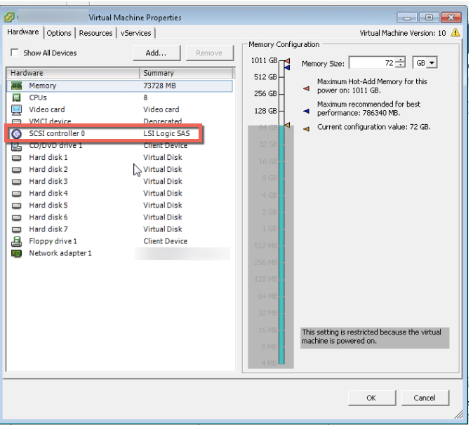
Once the new virtual disk is added you should see a new LSI Logic SAS SCSI controller is added as shown below.
Next highlight the adapter and select “Change Type” in the top right hand corner of the window and select Paravirtual. Once this is complete you should see similar to the below:
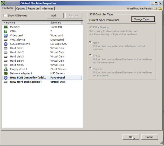
Next hit “Ok” and the new Controller and virtual disk will be added to the VM.
Now we open the console of the VM and open Compute Management and goto Device Manager. Under Storage Controllers you should now see VMware PVSCSI Controller as shown below.
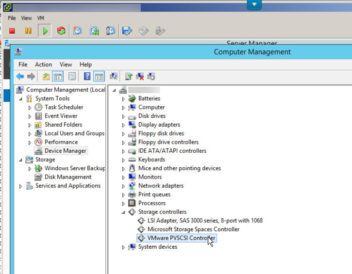
Now we are safe to Shutdown the VM.
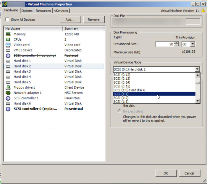
Once the VM is shutdown, Edit the VM setting and highlight the SCSI Controller 0 and select Change Type as we did earlier and select Paravirtual. Once this is done you will see the original controller is replaced with a new controller.

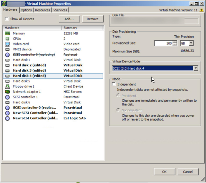
Now that we have the boot drive change to PVSCSI, we can now balance the data drives across up to four PVSCSI controllers for maximum performance.
To do this, simply highlight a Virtual Disk and drop down the Virtual Device Node and select SCSI (1:0) or any other available slot on the SCSI (1:x) controller.
After doing this you will see new SCSI controllers appear and you need to change these to Paravirtual as we have done to the first controller.
For each of the virtual disks, ensure they are placed evenly across the PVSCSI controllers. For example, if you have a VM with eight virtual disks plus the OS disk, it should look like this:
Virtual Disk 1 (OS) : SCSI (0:0)
Virtual Disk 2 (OS) : SCSI (0:1)
Virtual Disk 3 (OS) : SCSI (1:0)
Virtual Disk 4 (OS) : SCSI (1:1)
Virtual Disk 5 (OS) : SCSI (2:0)
Virtual Disk 6 (OS) : SCSI (2:1)
Virtual Disk 7 (OS) : SCSI (3:0)
Virtual Disk 8 (OS) : SCSI (3:1)
Virtual Disk 9 (OS) : SCSI (0:2)
This results in two data virtual disks per PVSCSI controller which evenly distributes IO across all controllers with the exception being first controller (SCSI 0) also hosting the OS drive.
What if I have problems?
On occasions I have seen problems with this process which has resulted in VMs not booting, however these issues are easy to fix.
If your VM fails to boot with a message like “Operating System not found”, I suggest you panic! Just kidding, this is typically just the boot order of the Virtual machine has been screwed up. Just go into the bios and check the boot order has the PVSCSI controller showing and the correct virtual disk in first priority.
If the VM boots and BSOD or crashes and goes into a continuous reboot loop then power off the VM and set the first SCSI controller where the boot disk is running back to LSI. Then reboot the VM and make sure the PVSCSI driver is showing up (if its not you didn’t follow the above instructions) so go back and follow them so the PVSCSI driver is loaded and working, then shutdown and change the SCSI controller back to PVSCSI and you should be fine.
If the VM boots and one or more drives do not show up in my computer, go into Disk Manager and you may see the drives are marked as offline. Simply right click the drive and mark it as online and reboot and you’re good to go.
Summary:
If you have made the intelligent move to virtualize your business critical applications, firstly congratulations! However as with physical hardware, Virtual machines also have optimal configurations so make sure you use PVSCSI controllers with multiple virtual disks and have your DBA span the database across multiple virtual disks for maximum performance.
The following post shows how to do this in detail:
Splitting SQL datafiles across multiple VMDKs for optimal VM performance
If the DBA is not confident doing this, you can also just add multiple virtual disks (connected via multiple PVSCSI controllers) and create a stripe in guest (via Disk Manager) and this will also give you the benefit of multiple vdisks.
Related Articles:
1. Peak Performance vs Real World Performance
2. Enterprise Architecture & Avoiding tunnel vision
3. Microsoft Exchange 2013/2016 Jetstress Performance Testing on Nutanix Acropolis Hypervisor (AHV)